My Online Retirement Calculator

Well, I’ve been retired for 3 months and looks like I’ve landed a contract starting next week.

I’ve been working on an online calculator and it’s now in a reasonable state. It’s lacking a lot of features that I would like, but I’ve run out of time for the moment. If you have a look, I think you’ll agree it has a lot more features than other available Australian online calculators already. Putting in this additional flexibility has been quite time consuming, and adding features has the potential to as well!

Rather than putting the whole project on ice, and waiting until it is perfect (i.e. never!), I’ve decided to put it out there. Some important caveats are that this calculator is really for people approaching retirement and wanting to find out when is the best time to retire. It’s also been developed under Google Chrome desktop, and this is the best means of running it (I don’t have the resources to do extensive testing!). The program is a BETA version and it’s also my first Javascript program!. If you spot any issues, please let me know!

I have found the existing calculators lacked precision, so have made this one more exact (e.g. it asks you the day you intend to retire, your birthday etc). Don’t be too put off with this, as you can change them later with sliders in the main page. You can also see how your assets change, and there is a numeric table which accompanies the graph. In addition, there is a “Mortality” graph which shows you the probability that you (and your partner if relevant) will be alive.

I’m not going to dwell on the calculator, other than to show, once again, how it relates to our situation!

Here is the graph showing expenditure by age. I assume we will live to 90, and we sell the investment property around September 2040. I’m already seeing a benefit here because previously my spreadsheets did not allow the sale of the investment property. Selling it makes sense as it can significantly increase the spend levels.

Note that when we sell the investment property, the funds go to cash. Later versions will allow this to go into another asset class. The same with if your super exceeds the 1.6M cap when you retire; excess will go into cash rather than, for example, remaining in the accumulation account or going into an ETF or similar.

And here is the graph showing the financial assets.

Here is the graph showing the mortality information.

Have a go and if you have any feedback, please let me know.

The 2018 Federal Budget

This post provide a quick overview of the 2018 Federal Budget as it relates to pending or actual early retirees. Not many measures impacting early retirees were announced in this budget, but those that were can only be described as beneficial. Let’s have a look at the most important ones.

The Pension Work Bonus

If you are on the Aged Pension, you can now earn an additional $50 per fortnight without a reduction in pension. We discussed the original pensioner earnings limitations in the Australian Super and Age Pension Rules post.

The Pension Loans Scheme

We discussed this in the Downsizing post. The Pensions Loans Scheme is a Government-run reverse mortgage scheme for pensioners, which, until now was only available under these circumstances:

• You (or your partner) must be over Age Pension age.
• You must have equity in Australian Real-estate.
• You must not be drawing the full age pension.
• Your ineligibility for the full age pension must not be due to both the assets test and the incomes test.

If you were eligible:

• The most you could receive is the difference between the Age Pension and your present part Age Pension (which may be zero). The amount is paid fortnightly (i.e. it cannot be taken as a lump sum) and is not taxable. So, for example, if you are not eligible for the Age Pension at all, you could receive up to the Age Pension.

As mentioned in the original post, these rules are pretty restrictive and would only really apply if you have illiquid assets in addition to your PPOR which you cannot access to cover living expenses.

In the new scheme, there is no longer the restriction that you are not drawing the full age pension, and also the amount that you can borrow is the amount that brings you up to 150% of the Age Pension. So, for a couple at present rates, this would be approx $53,360.

I predict that this scheme will be quite popular as the interest rate is lower than private schemes (but does have the restriction of the amount you can borrow, e,g, no lump sums).

Works Test and Super Contributions

In the Australian Super and Age Pension Rules post we mentioned that “you cannot make non-concessional contributions to Super if you are over 65 unless you pass the works test.”.  You can now contribute to Super during the first 12 months after 65 if your Super balance is less than $300K without having to satisfy the works test.

How will these measures affect us?

As usual, we will look at how these measures will affect us.

The new Pension Loans Scheme looks attractive and something we could use, depending on how long we are looking at staying in our current residence and how much funds we need. It’s something we would assess further into retirement.

The other measures don’t really impact us.

Conclusions

The 2018 Federal Budget does not have any major impacts on pending or actual early retirees. The most significant one is the updated Pensions Loans Scheme, which, depending on circumstances, could be quite attractive.

 

 

 

 

 

Risk and Return

In this post we look at the relationship between the riskiness of a portfolio and the corresponding expected spending patterns in  retirement. This will help with answering the question of what percentage of a portfolio should be in risky assets such as shares and what percentage should be in cash.

As usual I look at ourselves as a case study. In this post I look at one model of spending only. I assume we are a couple until 90, and then if we are still alive, we go onto the age pension only. At the end of each year, we work out the spending level for the next year by calculating the spending level for the remaining years that will make assets at 90 equal to zero, assuming the return on the portfolio for the remaining years is equal to the expected return, and spending is the same for each subsequent year (or in accordance with a specified spending pattern). This model has been discussed in previous posts.

If I have time, I will update the post to include mortality-based spending for the single person and the couple.

Portfolio Returns

For simplicity, in this post I assume that your portfolio is made up of shares and cash only. That is, there is no opportunity for further diversification into property etc.

In order to work out the returns and volatility of a portfolio with a certain percentage of shares and a certain percentage of cash, we need to know the returns and volatility for each of these asset classes.

For cash, I have assumed a real return of 0.5%, and a volatility of zero. That is, the bank will always give you 0.5% above inflation.

For shares, we need to look at historic returns. We did this back in the Retirement Calculations Post. Here is a graph that shows a 30 year moving average of real geometric returns (including dividends) for returns of the Australian Share market since 1953:

You can see that there is no overall trend for returns, and the average is around 8%.

And here is a similar graph showing a moving average for volatility:

You can see that volatility is increasing over time, and the average is around 17%.

If we have a mix of n% shares and m% cash, the return will be  0.08n + 0.005m, and the volatility will be n*.17.

Portfolios and Spending

We can now see what happens in our particular case if we invest  the proceeds of Super into various proportions of Shares and Cash.

Like the previous post, we use the staring position described in the Tweaks and Mathematical Diversions post, however now we use post-January 2017 age pension rates rather than pre-January 2017 age pension rates, and we will also use a more realistic spending drop of 1% per year from 65 through to 85.

The diagram below is an animation showing the spending patterns (note that in order to generate each individual graph, we only did 1000 runs, so it is not so smooth).

What is interesting here is that the average spend per year goes up quite a bit when we increase the proportion of shares, and there isn’t much downside. That is the likelihood of a low spend does not increase that much when we increase the proportion of shares.

The below graph should help with understanding this better. Note that the expected percentage of retirement below threshold statistic is a straight-forward average to 90 – that is it does not incorporate mortality data.

You can see in the graph that average spend increase quite a bit by increasing the percentage of shares (it nearly doubles if we increase the percentage of shares from 0% to 100%) and in most cases the expected proportion of retirement spent below various thresholds decreases when we increase the share ratio. An exception to this is the ASFA threshold, but there is only a minor increase.

The other interesting thing is that the expected percentage of retirement below the thresholds in the above diagram decreases sharply from a 0% to a  50% share percentage, and then drop off much more slowly.

Conclusions

In this post we have shown, under the assumption that share market returns for each year are normally distributed and independent, and follow historic averages, that it is sensible to have our Super assets invested in a portfolio with 100% shares. This portfolio mix provides the highest average spend, and offers very little downside over alternatives. This is a surprising result as most investment advisors advise reducing exposure to shares as you get older.

Mortality and Risk

Introduction

In this post we provide information on retirement spending patterns when presented with both investment risk and mortality. To date we have considered these separately. This post builds on the work in previous posts:

In the Retirement Calculations post we  worked out the spend per year assuming we are on the age pension only at age 90 and also assuming we would like a constant spend to 90 where possible (or at least a constant spend subject to specified percentage drop at various ages).

In the More on Risk post we worked out how our retirement average spending will vary if we assume annual Super returns vary independently according to a normal distribution and  the spend per year during each year of retirement is worked out by solving for a constant annual spend for remaining years while being on the age pension only at age 90. As an aside, in the ALP Super Tax post we showed how the spending each year will vary (rather than just the average).

In the Mortality post we got rid of the assumption that we need to be on the aged pension only at 90, and instead assumed that in order to work out our spending for a given year, we would assess our likely longevity at the end of the year and spread our remaining funds from the present age to a longevity-dependent future age.

In this post we combine the concepts in the Mortality and More on Risk posts.

Because we are getting into some serious number crunching territory now, I will focus on the Single person.

Single Person – Mortality and Risk

In the Tweaks and Mathematical Diversions post we worked out the spend per year using us as an example, commencing in 2015 and using pre-January 2017 age pension rates. We also assumed a drop in spending at 70 of 10% and another drop at 80 of another 10%.

The below graph is an update, now showing for a single person rather than a couple, using post-January 2017 age pension rates rather than pre-January 2017 age pension rates, and also using a more realistic spending drop of 1% per year from 65 through to 85. You can see that there is very little aged pension!

Now, lets assume that Super returns are normally distributed, with a volatility of 6.21% (the same volatility we assumed in the More on Risk post). The graph below shows the variation in the spending per year for each age. The green band represents 60% of the outcomes and the blue + green band 80%. That is 60% of the time the spend per year will fall within the green band, and 80% of the time the spend per year will fall within the green + blue bands.

You can see that as time goes on, there is more uncertainty about the spend per year. Also, because we only have access to cash to 60, there is not much variation prior to 60.  Because we only have access to a limited amount of Super prior to the house sale, the variation prior to 64 is also less than after 64.

Now lets look at spending assuming we take in to account mortality. The graph below shows the spend per year assuming we moderate spending according to mortality information, and the spend per year is based on spreading funds from the present date to the whereby we will only be alive with a probability of 10% (for a male).

You can see that our drop in spending continues beyond 85 because of the reduction due to ageing and the spend per year falls below ASFA comfortable about 96.

Finally we can now show the mortality-based graph taking into account volatile super returns:

You can see that at around 89 90% of the time our spending will be above ASFA comfortable, while at 98 90% of the time our spending will be below ASFA.

Couple – Mortality and Risk

The below graph shows the spending for a couple, assuming we run out of funds at 90, and again we reduce spending by 1% from 65 to 85.

Here is the graph showing the variation in spending assuming variation in Super returns.

We can also show how spending for a couple varies when we plan to reduce our spending in accordance with our expected longevity. However, we are in some serious number crunching territory now, so this will need to wait until later!

Conclusion

We can combine the spending approach described in the mortality post with the approach used in the More on Risk post to show how mortality-based spending is likely to vary if we introduce super return volatility. This may be a useful graph to display on an interactive web site.

In the next post we will look at how spending varies with the riskiness of our investment portfolio.

Downsizing

Many pending retirees are planning to downsize in retirement. Downsizing has the benefit of releasing funds from the sale of the family home. Other potential benefits including moving to a home which is easier to maintain and also moving to a location more suitable for retirement.

There can be disadvantages to downsizing however.  Downsizing often involves moving out of a familiar and desirable neighborhood and away from friends and relatives.

This post looks at financial strategies which can help retirees who would like to delay downsizing. Specifically we look at private and public sector Reverse Mortgages and also Home Reversion schemes.

As usual, we will use ourselves as case study.

Our Example

Let’s look at our case. In the 2016 in review post I updated a plan whereby we will sell the family home and move into another already owned property in a seaside town.

To recap:

• I am married with no children, and am now 54. We are Australians but living overseas at the moment. We intend to come back to Australia at some stage (present date unknown!). The plan assumes we retire in early 2017, although this may change.
• We own a house in a capital city which we intend to sell when I get to 64. Some of the house sale proceeds will go into superannuation at this time using the bring forwards rule, and remainder will go into cash.
• We own an investment property.
• We have Super and Cash assets.
• Another property in a seaside town is a possible inheritance. This plan assumes that we move into this property when we sell our main residence, and it only becomes available to us at this time. However, if this does not eventuate, we will move into our investment property. This plan assumes the former, but the latter will have similar outcomes.
• We intend to spend 10% less when we get to 70, and another 10% less when we get to 80. This reflects our likely spending requirements.

Here is the estimated spending pattern under this plan (with 2015 and 2016 shown as actuals):

You can see the age pension becoming available at around 84. You can also see that our annual expenditure over the last 2 years has been very low (less than $40k!).

Here are the assets (in 2017 dollars), with actuals from 2014, 2015 and 2016:

You can see the house being sold at 64, and some of the assets going into Super and some going into Cash (now that the non-concessional limit has been reduced, as per the 2016 budget, not all of the funds can go into Super).

Now, let’s assume that we want to delay the sale of the house and the move to another location (aka Downsizing). In the absence of any additional strategy, this will involve a lower level of spending prior to selling the home, and a higher level afterwards. Here is an updated plan assuming we delay the move by 10 years and that we don’t leave until 74:

You can see that we are now eligible for the Age Pension at 67, ineligible again at 74, then eligible again at 84. Also, due to the limited amount of liquid assets prior to 74, our spending prior to 74 is lower than after 74. Ideally we would like to spend more in early retirement and less in later retirement in accordance with our chose spending pattern (10% less at 70, and another 10% less at 80) and we can no longer do this. Still, the spending levels are perfectly acceptable to me at least!

Here are the corresponding assets:

Note that I have assumed that the bring forward amount coming from the house sale can be invested in Super like assets. This should be a reasonable assumption given the SAPTO offset, but to understand the implications of this approach fully, a probabilistic approach would have to be used (refer here for an example).

Also, you can see the Super (and Cash) running out just prior to the house sale.

Here is a more extreme example whereby we plan to delay the move to 80:

You can see that expenditure prior to 80 is quite a bit lower than the spend in other plans.

Reverse Mortgages

One strategy to help delay the house sale while at the same time minimizing the impact on funds available for spending is based on the use of Reverse Mortgages. While Reverse Mortgages have received a lot of adverse publicity, regulations on these types of products have recently improved, and there are some real advantages. Firstly and most importantly you can access the equity in your home without having to sell it. Also, most reverse mortgage products allow you to access the equity in your home as an income stream or on an as-needs basis. That is, you don’t need to access the funds as a lump sum. This means that the income source from your home should not impact your Age pension, and also you only pay loan interest on the funds you have drawn. Finally most reverse mortgage products stipulate that there can be no claims on your other assets if you end up owing more on your reverse mortgage than your home is worth, and you cannot be forced to leave your home (this is known as the “no negative equity guarantee” or NNEG).

Disadvantages or include a high interest rate (which might be expected due to the longevity risk worn by the financial institution), the fact that you can only mortgage a percentage of your home (the percentage normally increases as you age) and the need for close management of the loan as the amount owing can increase quickly due to compounding (especially as the interest rate is variable and not fixed).

SEQUAL is an industry association that promotes home equity products and the maintenance and enforcement of strong consumer protection principles for the industry and it is generally recommended that you choose a product from a participating member.

So, lets take a look at how a reverse mortgage would work. I am using as an example the Commonwealth Bank product. At the time of writing, this product allows a reverse mortgage of between 20% (if aged between 65 and 70) and 40% (if over 85) of the value of the family home (this percentage is known as the Loan to Value Ratio or LVR), with overall maximum limits of between $275K and $425K. The annual interest rate charged is 6.37%. As the level of detail in the CBA pdf is not that great, I have made certain assumptions about the product. Refer here for these.

Here is the diagram showing the spending patterns if we sell the family home at 74, and take out a reverse mortgage that commences at a time that results in our spending patterns being leveled out. I have assumed an interest rate of 6.37% throughout the mortgage.

You can see that there is no increase in spending after selling the house and we maintain the 10% reduction at 70 and 80. Under the plan, the reverse mortgage value gets to about 19% of the house value. The total real (2017 dollars) of the amount borrowed is $257K. If we borrow more than this then spending prior to selling the house is too high, and if we borrow less, then it is too low.

Here is the diagram showing the assets (real values):

I have again assumed for the purpose of this post that I can contribute the bring forward amount of house sale proceeds to Super-like investments.

Note that the light Blue House Value is the value nett of the outstanding reverse mortgage amount. You can see the value declining near the time it is sold.

You can also see that during the period between taking out the reverse mortgage and selling the house there are no super or cash assets.

What about if we wanted to stay until 80?

Well, this is more complicated because the optimal solution involves borrowing more than the upper limits imposed by the CBA product. Here is the optimal solution, assuming there are no limits on how much we can borrow against the mortgage:

In this solution, the Reverse Mortgage gets to about 53.5% of the house value, and the real amount borrowed is approx $602K.

And here is the solution within the CBA limits:

Here the real value borrowed is approximately $272K. Note that this is  less than the $325K available if we started the loan at 74 because of the interest charged and also the discounting of the value of the loan by inflation.

What about another Reverse Mortgage!

It is possible to reverse mortgage our downsized second home in order to release another income stream. This would elevate spending again. If we are over 85, we could release 40% of the house value and this could feed into higher spending prior to 85.

Would we want to do this, if so when, and what are the disadvantages?

Here is the diagram for the second reverse mortgage, assuming we take it out so that drawdown funds are available up until 90, and assuming that we sell the house at 74:

You can see that the funds released in the second reverse mortgage mean that the first reverse mortgage cannot bring forward enough funds to maintain our spending pattern. i.e. after the house sale our spending will now increase rather than remain flat.

Also, at 90, we are living on the Age Pension. As described in the mortality post,  at the age of 87 it is more realistic to assume that we will live past 90, so a lower spend should be planned for. It is possible to combine this post with the mortality post to work out when it is best to take out a reverse mortgage assuming a plan based on expected longevity. I might do this later!

There is one significant advantage and one significant disadvantage to a second reverse mortgage.

The significant advantage is that the reverse mortgage never needs to be paid back because we will not be moving to another home.

The significant disadvantage is that there is potentially a small (or no) residual to be paid to any  beneficiaries on death, and also, in the event that one of us needs to go into Aged Care, the lack of a property may impact on the quality of the Aged Care service. I’ll do a post on Aged Care soon in order that we can understand this better.

Using the Reverse Mortgage as described above, here is reverse mortgage value as a percentage of the house value.

So, for example, if we were go into Aged care at 94, approximately 50% of the house value would be available to fund Aged Care.

The Pension Loans Scheme

There is an alternative to the private sector reverse mortgages. The Pensions Loans Scheme is a scheme administered by the Federal Government and has the following characteristics:

In order to be eligible:

• You (or your partner) must be over Age Pension age.
• You must have equity in Australian Real-estate.
• You must not be drawing the full age pension.
• Your ineligibility for the full age pension must not be due to both the assets test and the the incomes test.

And:

• The most you can receive is the difference between the Age Pension and your present part Age Pension (which may be zero). The amount is paid fortnightly (i.e. it cannot be taken as a lump sum) and is not taxable. So, for example, if you are not eligible for the Age Pension at all, you could receive up to the Age Pension.
• The fortnightly interest rate is 5.25% (effectively 5.4% annual rate). According to this article, the rate is fixed.
• You can continue to borrow while the value of the loan is less than Age Component Amount * (Value of Realestate Assets – Guaranteed Amount)/$10,000. The Guaranteed Amount is the amount  that you wish to retain on death. If you have more than one property, you can choose which to use in the assessment for a loan.
• You can find the Age Component amount here (buried in the act documents!). Effectively you can borrow from 17% (at 55) to 67% (at 90).
• You must pay back the loan when you die or when you sell the home.
• I couldn’t find anything on the no negative equity guarantee (i.e. there can be no claims on assets outside the collateral in the event that the loan exceeds the value of the collateral). However, I believe that this would apply.

Could we use this type of loan and if not, for whom would it be attractive? Under this loan, the most income per year you can receive is the Age Pension. This assumes that you are not eligible for the any Age Pension e.g. you have at least $823K in assessable assets. Or if your assets are lower,  you could receive a lower amount. The problem is, if you have these assets, you are unlikely to want to take out a loan and pay the loan interest rate! i.e. it would be more sensible to use your assets for living expenses rather than taking out a loan, but if you do this, you eventually become ineligible to take out the loan!

Seems to me that there aren’t many circumstances where this loan would be attractive. Maybe it has been deliberately made so in order not to compete with private sector products. Some people have recommended that the Age Pension eligibility criterion be removed for this product.

Home Reversion Schemes

Home Reversion Schemes are another type of scheme which permits pensioners to access equity in their homes. The idea behind this type of scheme is that you can sell a proportion of your home for a lump sum. When you sell your home, go into aged care, or die, the vendor of the product receives the agreed percentage of proceeds.  The lump sum you receive is a proportion of the percentage value of the home, with the proportion getting larger the older you are.

There is only one vendor of Home Reversion Schemes in Australia, Homesafe. The characteristics of their scheme are:

• The scheme is only available to home owners in some postcodes of Sydney  and Melbourne.
• You must be over 60.
• The land value of the property must be at least 60% of the value of the property, as assessed by an independent valuer.
• The maximum percentage of the home that can be sold is 65%.
• Normally the lump sum is between 35% and 65% of the percentage of the value of the home at the time the contract is signed. This will normally vary according a number of parameters, one of the most important being age.
• You retain title in the home.
• Because you receive a lump sum, this may impact on your pension.

The percentage of the house value that you receive is not published, so it is difficult to assess what kind of deal you are getting. Assuming that you don’t leave the family home, then this is equivalent to receiving a lump sum injection while sacrificing a percentage of the home for use in Aged Care or to leave to beneficiaries. Further modelling for our own situation would be dependent on availability of percentage discounts assigned to the house percentage.

Vendor Risks

It is interesting to look at the vendor risks for these types of products.

For the Reverse Mortgage product, the main risk is that the value of the outstanding loan becomes higher than the value of the property. This is more likely to occur where the property value declines or does not increase as fast as expected, the owner remains in the property for a longer time than planned, or interest rates increase to a higher level than planned. These are mitigated to some extent via the aged-dependent Loan to Value Ratio, a higher than normal interest rate, and also, where the loan is taken progressively, including the interest in the amount that can be loaned.

For the Home Reversion product, the main risk is that the value of the lump sum is not recovered (with interest) when the home is sold. This is more likely to occur in the same set of circumstances, i.e. the . property value declines or does not increase as fast as expected, the owner remains in the property for an especially long time, or interest rates increase to a higher level than planned. These risks can be mitigated by ensuring the percentage of the home given as a lump sum is appropriately discounted.

Conclusions

If you are planning on downsizing to help finance your retirement, the use of private sector Reverse mortgages can help with extending your stay in the family residence. We have shown that in our case, under certain assumptions by using Reverse  Mortgages we can delay the move from our family home by about 10 years with only minimal impact on spending patterns.

The Federal Government also offers a type of Reverse Mortgage service, however there are very few instances where this services is likely to be useful.

Home Reversion Schemes may also be of help to the retiree, especially when you want to quarantine a proportion of your home for beneficiaries or help with Aged Care.  It has not been possible to model how we could use a Home Reversion product because not all details are available/published.

Would I use one or more reverse mortgages?

Comparing my original spending plan with the plan using two reverse mortgages, the spending levels are roughly the same, except that in the latter, I can maintain spending levels and leave my home in 20 years rather than 10. Still, I would prefer not to manage a reverse mortgage if I didn’t have to, and having a sightly lower level of spending may be an acceptable trade-off (so the plan to leave at 74 without a reverse mortgage, which only involves a $10K reduction in spend prior to the house sale may be perfectly acceptable). The risk of interest rates going higher, and the capital in the home disappearing quickly is a real one, and something I would prefer not to deal with.

I think I will see how are our actual spending levels pan out in the first years of our retirement and if there is a real need for additional funds to see if a reverse mortgage is likely to make sense.

(*) The information on the CBA website is a bit light on details. I placed a few calls to CBA, but call center staff were not that knowledgeable either and suggested an appointment at a branch!

I have made some assumptions to help with the analysis. The general principles in this blog should remain valid, but if some of the assumptions prove incorrect, there may be need to be some minor adjustments.

I assumed:

• The Bank will continue to loan you money while the outstanding value of the loan is less than the maximum limit. If you take the loan as a lump sum, then this means you can borrow the full amount of the maximum limit. However, if you take the loan progressively,  then you can only continue to draw down funds while the outstanding value of the loan is less than the maximum. As the outstanding value will increase due to interest and fees, and the real maximum value declines over time, this effectively means the real value that you can borrow will be less than the nominal maximum amount. I have based this assumption on the somewhat cryptic comment in the CBA product pdf: “Should the borrower/s choose to draw down the facility on a periodic basis, the full amount of the facility limit may not be available due to the capitalised effect of interest and fees.”
• The loan limit applicable is the limit at the time you took out the loan. That is, if for example, you have an outstanding reverse mortgage loan and you turn 85, you don’t get access to more funds reflective of the increased maximum loan at this age.
• I didn’t factor in any fees other that Interest. That is, I didn’t factor in setup fees, withdrawal fees (if any) etc. These should only have a minor impact on the overall result and introduce unwanted complications.
• I assumed maximum loan limits increase with inflation, although once the loan is taken out the limit is fixed.

Note that:

• I have worked out the amount owing on the loan based on similar techniques described in the “Mathematical Diversions” post.
• The total amount owing on the loan can be a lot more than the loan limit because there is no fixed date for paying it back. This is why the bank limits the amount you can borrow and this varies by age!

Analysis of the ALP Super Plan

In this post I take a look at the Super plan that the ALP has proposed to be implemented should they be elected into government. This analysis is especially timely as the 2016 Australian Federal election is approximately one month away, and significant changes to the Super system were recently announced by the LNP government as part of the 2016 Federal Budget. These LNP changes are unlikely to be become law if the ALP wins the Federal election.

What is the ALP Super Plan?

Information on the ALP Super plan may be found here.

The first section of this site describes a policy that taxes Superannuation returns in Pension mode in excess of $75,000 at 15%. The information on the ALP site is actually quite confusing (perhaps deliberately so) because it first states:

“The proposed measure would reduce the tax-free concession available to people with annual superannuation incomes from earnings of more than $75,000. From 1 July 2017, future earnings on assets supporting income streams will be tax‑free up to $75,000 a year for each individual. Earnings above the $75,000 threshold will attract the same concessional rate of 15 per cent that applies to earnings in the accumulation phase.”

and then states:

“This measure will affect approximately 60,000 superannuation account holders with superannuation balances in excess of $1.5 million”

These statements are inconsistent because you may very well have significantly less than $1.5M in superannuation assets but still have more than $75,000 in superannuation income for a particular year. In fact this is quite likely because the average Super fund typically returns in excess of the 5% assumed by the ALP (e.g. the Australian Super balanced fund has averaged 8.69% per year since 2004, and this includes the GFC).

The $75,000 threshold appears not to be indexed to inflation. Most commentators (e.g. here, here and here) have concluded that the $75,000 is not proposed to be indexed, although some have speculated otherwise (e.g. here). To quote from the second commentary:

LABOR’S proposed superannuation tax on wealthy retirees could eventually hit more older Australians because it will not be automatically indexed to inflation.

…

Opposition treasury spokesman Chris Bowen yesterday said a future Labor Government would consider lifting the $75,000 threshold when necessary but dismissed automatic indexation.

“I would expect any government of the day would monitor the thresholds to ensure that the original policy intent was being met and would respond accordingly,’’ Mr Bowen told the National Press Club.

For the purposes of this post, I have assumed it is not indexed. Should authoritative information become available which contradicts this assumption, I will update the post.

The second part of the site describes a plan to reduce the Higher Income Superannuation Charge (HISC) threshold from $300,000 to $250,000. I won’t look into this second part as it will not impact many Australians (and a similar policy is already part of the LNP Plan).

Who will be impacted by the ALP Plan?

The ALP plan looks fairly benign (after all, not many people have over $1.5M in super), but we will investigate to see if this is actually the case. The policy can and will impact many people with considerably lower balances than $1.5M because:

• Super returns are, on average, higher than 5%.
• Super returns are not the same every year, but actually have a fairly high variation. During the years that Super returns are high, the government of the day will collect a high tax from Super members, while when the returns are negative, the retiree will suffer the losses with no compensation. An example I provided earlier may be found here.
• The $75,000 limit is not indexed. So, the $1.5M limit (which will actually be smaller in any case if the average return is used) will diminish overtime. The process will be accelerated when we move away from the present historically very low inflation rates.

How to mitigate against the effects of the policy

The obvious mitigation to this policy for a couple is to split Super between individuals. That way each individual essentially receives half of the returns, and there will be less likelihood of being subject to the tax. This kind of splitting is likely to be less easy under the new LNP rules regarding non-concessional limits (should they become law).

Another mitigation is to move some of your funds outside the Super system. In 2016, income below $18,200 per year is tax free. Furthermore if you are above retirement age, SAPTO allows, in 2016, a tax rebate of up to $57,948 for a couple. If you have funds in the super system and believe that you may be subject to the tax, then you could place some of your funds in, for example, a combination of cash and index trackers such as this one.

As an example, say you are below retirement age but over 60, have $2M in super, the Super rate of return for the year under analysis is 10%, and the Index funds/Cash combination you invest in also returns at this rate:

Tax without Super Splitting, No index fund: $18,750

Tax with Super splitting, No index fund: $7,500

Tax with Super Splitting, $500,000 in Index fund: $2,584

Tax with Super Splitting, $364,000 in Index fund: $2,040

Note that the latter is the optimal (retrospective) solution for a 10% return. By making assumptions about the distributions of returns from Super and the Index fund, it would be possible to provide a recommended optimal mix between the Super fund and the Index fund. If the ALP form a government in 2016, I may do this in a later post.

Further mitigation strategies would include postponing selling your (tax exempt) PPOR until existing Super assets are reduced.

See here for more information on mitigation.

An Analysis of our Situation

As usual, I will look at how this policy will impact on us.

I will look at the impact of the tax through three models, increasing in order of sophistication and realism, and also compute power!

Model 1 – Assumes a constant Super return each year with no variation, and a constant spend. This is the model used by the ALP when determining the impact of the tax.

Model 2 – Assumes a constant spend and variable Super return.

Model 3 – Assumes a variable Super return and a spend that is calculated at the end of each year that would result in Super being zero at 90 under the assumption of standard inflation and Super returns for remaining years.

Model 1 – Constant Super Return with no variation

In this section I will assume a constant Super return of 5.5% in the accumulation phase and 6% in the pension phase, as per the analysis described in the Tweaks and Mathematical Diversions post. At 6%, we would need more than $1.25M in the Super pension phase account to be subject to the tax.

Here is the spending plan prior to the tax, this time showing, for the purposes of comparison, the tax in accumulation mode.

Super Returns are always the same, no Super splitting

If I  deduct 15% of any earnings above $75,000, as per the ALP Super tax without Super splitting, it appears that the policy is fairly benign. Here is the spending plan with the ALP tax policy in operation:

As you can see, there is not really too much difference (about $700 per year).  Total ALP Super tax is approx $25.6K in 2015 dollars and to get back to our original spend, we would need an additional approx $30.5K.

Super Returns are always the same, Super splitting

OK, what if we split Super between accounts? Well, in this case there is no impact because Super is always below $2.5M, the amount that would be required to cause tax to be levied, assuming a 6% return.

Super Returns are always the same, Effect of Inflation

Unlike most other policies, the ALP Super Plan is impacted by higher inflation, so let’s see what happens when the rate of inflation increases.  We can expect a higher tax as the $75K is not indexed. In addition, Super returns will be higher, so we can expect higher taxes.

Here is the diagram with no Super splitting, and assuming an additional 3% inflation becomes the norm, for a total of inflation rate of 5.73%. Total ALP Super tax is now $145K in 2015 dollars. As you can see, this is quite significant when compared to the accumulation tax.

And here is the same diagram, but now assuming we split Super. Total ALP Super tax is now approx $77K in 2015 dollars.

The diagram below shows the effects of various inflation rates. For reference, and as a sanity check, the spend with zero tax is also shown. As expected, spend does not change much with increasing inflation without the tax.

And here is information on the historic inflation rates in Australia (from the ABS site). You can see that inflation has been pretty stable since about 2001.

Note the region between the two horizontal bars is the RBA target range for inflation.

Model 2 – Constant Spend and Variable Super Return

Now lets take a look to see what happens when we have variable returns. We can expect higher tax and lower spend when we take into account variable returns, because the Super member will get hit for higher taxes in the good years, and will not be compensated in the bad years.

Luckily an analysis of the impact on retirement of variable returns has already been completed in the More on Risk post. In this post we looked at, amongst others, the impact of variable super returns on the length of time that Super would last assuming a constant spend.

Here is the graph showing the distribution of ages at which funds run out, assuming there is no tax as described in More on Risk. I have used, for the moment, the Age pension rules prior to the 2015 budget changes as described in this post. Note that the spend levels here are the spend levels which cause Super at 90 to be zero assuming no Super return variation (which is an average spend level of $90,463, as described here):

Note that the average age is 90.36. I have colour coded showing the 60% of results that are less than 20% percentile and higher than the 80% percentile as green , and the 80% of results which are less than the 10% percentile and higher than the 90% percentile as green and blue.

The diagram below provides summary data for a number of scenarios using the colour coding above:

And here is similar information for the amount of tax:

Constant Spend, Super Returns are variable, Sensitivity to Volatility

As Super returns become more volatile, we can expect the average age funds will last to be reduced. This is indeed the case.

Here is how the Age at which funds run out varies as we increase volatility, assuming this time we split super, and spend at the rate where we solve for super being zero prior to the 2015 budget changes and any taxes:

You can see that the average age to which funds last declines as volatility increases, but not significantly so.

And here is the average total ALP Super tax (in 2015 dollars) by volatility:

Note that the volatility of the Australian Super Balanced fund returns over the last 17 years is about 7.5%, and the volatility of the Vanguard ASX Index fund over the last 10 years is about 21%.

Finally, here is the Age funds last until by Volatility without the Tax:

You can see that the average does not vary much, but total variation increases quite a bit.

Constant Spend, Super Returns are variable, Tax by Age

The diagram below provides details of the average ALP Super tax by Age when assuming variable returns, and also assuming we do not split Super. The spend levels are those which make Super at 90 equal to zero for the standard fixed returns of 6.0% and the ALP Super tax without splitting. For comparison, I have included the taxes for the fixed returns. Total ALP Super tax for variable returns is about $75.5K, while total tax for fixed returns is about $25.6K. I have assumed post 2015 Budget pension rates.

Here is the distribution of the amount of tax by age. Note that I have not included the zero tax possibility in the diagram as this would tower over the other probabilities (in most years zero tax is paid after 64):

Model 3 – Variable Super return and a spend that is calculated at the end of each year to make Super zero at 90.

OK, before we start modelling the ALP Super Tax increases with model 3, let’s look at the results of this model with the updated pension rates (the More on Risk post had the old pension rates). I will also present the results of this model in some different ways:

Here is the spend per year for this model using the new pension rates:

Here is a graph showing the spend in more detail, this time including the full distribution for each year:

The result is not so smooth as only 4000 runs were done.

OK, let’s take a look at the results for the ALP Super tax. The graph below shows the average spend for the spend prior to the 2015 pension changes, after the changes, the ALP super tax with splitting, without splitting, and without splitting and 5% inflation:

And there are the taxes for the last three policies:

 

Why I dislike the ALP Super Tax!

The ALP has given two reasons to support the introduction of their Super Tax:

1. The majority of the Super Tax concessions go to the top income earners, and these concessions are unlikely to reduce future Age Pension expenditure significantly.
2. The cost to the Tax payer for the Super Tax concessions in the form of forgone revenue is large and growing and is not sustainable.

The ALP Super Tax will indeed have the effect of reducing Super tax income concessions in Pension mode to top income earners, and this is a good thing. However, it will not impact the Super accounts of these same people when in accumulation phase (unlike the LNP policy, which restricts the amount that can be contributed).

The Tax will also have the effect of gradually affecting more and more people as the $75K limit is eroded by inflation, eventually affecting everyone. In addition, significant chunks of people’s life savings will be eroded in the event of high inflation or high market volatility, both of which are outside the control of the retiree. The government will gather more tax, and more people will be find themselves on the Age Pension sooner. The tax is a disincentive to getting ahead, not only for high income earners, but also for average person.

Conclusion

When I started this post, I suspected that the ALP super plan would have a significant impact on people like me, mainly because of the high taxes in high return years. I gave an example to show how this would work. In order to better understand the impact of the tax on us, I have used three models:

• In the first model, I assumed that Super returns are always the same, and solved for Super being zero at 90. I looked at splitting and not splitting super funds between individuals in a couple, and also looked at the impact of an increase in inflation.

• In the second model, I assumed that Super returns are normally distributed and the spend per year (adjusted for inflation) is static. I worked out how the age at which Super funds run out is impacted, and how much additional tax is due. I looked at splitting and not splitting super funds between individuals in a couple, and also looked at the impact of the Super return volatility.

• In the third model, I assumed that Super returns are normally distributed and the spend to be used for each year is worked out in advance as the value that makes Super at 90 zero, assuming a constant spend and standard rates for Super and inflation for remaining years. I looked at splitting and not splitting super funds between individuals in a couple, and also looked at the impact of 5.7% inflation.

These models showed that in our situation:

• If we do not split Super between accounts, the ALP super plan will result in an additional tax of $25.6K (model 1), $66K (model 2) or $68K (model 3).
• Super splitting can significantly reduce tax ($25.6K to zero in model 1, $66K to $27.8K in model 2 and $68K to $25K in model 3).
• Tax to be paid and average spend is very sensitive to increases in inflation. The higher the inflation, the more real tax to be paid and the less to spend. Tax goes up quickly with inflation increases.
• Tax to be paid is also sensitive to Super return volatility, although quite a bit less sensitivity than to inflation. The more volatility, the higher tax to be paid.

Given the sensitivity to inflation, and the inability of the retiree to influence it, it would make sense to index the $75K threshold to inflation.

 

 

 

 

 

 

 

 

 

 

The 2016 Federal Budget

Well, it seems that the Government of the day can’t resist tinkering with the Super and Pension system during each federal budget. In 2016 the LNP Government is no exception, and in fact, there have been some major changes in the 2016 Federal Budget. In this post I will describe how the most relevant changes will impact retirees, early retirees and, continuing with the theme of using us as a case study, our situation in particular.

I will also look at some interesting aspects of the changes, and also have a brief look at the ALP alternative.

Reasoning behind the Changes

The government has made clear that it believes that the purpose of the Super system is to:

• Assist retirees to obtain the assets required to enjoy a comfortable retirement
• Reduce the cost to the government of providing retiree support by providing incentives to people to contribute towards their own (no more than “comfortable”!) retirement.

According to the government, it is definitely not supposed to:

• Provide tax-free income on earnings in retirement where those earnings are in excess of the amount required for a retiree to achieve a “comfortable retirement”.
• Provide assistance to retirees to accumulate assets in excess of the amount required to achieve a “conformable retirement”

Of course, a “comfortable retirement” is a relative term, but the government has sought to define the amount of income required to achieve it via this legislation.

Note that it is perfectly possible for a person to enjoy a retirement with more funding than the funding required for the government defined “comfortable retirement”, it’s just that the retiree will not receive any tax benefits for the excess funding.

In view of the above,  a raft of measures have been introduced in this budget  aimed at reducing existing large (tax-free) pension-mode Super accounts and, moving forwards, making it difficult for individuals to transfer excessive amounts of funds into the Super system (including the low tax accumulation accounts).

To my mind, these measures are very sensible and long overdue. In Australia today there are some individuals with over $100M in their Super account. Why should the community be supporting the tax free returns generated by these extremely rich individuals?

What are the major changes that will impact early retirees

There are four major changes that will impact on early retirees. These are:

A Cap of $1.6M on the amount that can be transferred to retirement phase accounts

Retirement phase accounts are the so-called account based pensions. This measure is saying you can transfer no more than $1.6M from your accumulation account into your account based pension. Note that normally you are eligible to do this at 60, and most people will do this as soon as possible in order to reduce the accumulation mode tax (normally around 8%) to zero.

Although not stated in the budget papers (page 40 onwards), according to this web site, it seems that the $1.6M cap will be indexed  “in $100,000 increments in line with the Consumer Price Index, similar to the treatment of the age pension assets threshold.”. It would be good to see a government site confirming this.

If you wish to make multiple transfers into your account based pension (e.g. if you sell your house, or receive an inheritance), you can do so.

According to the budget papers:

“The amount of cap space remaining for a member seeking to make more than one transfer into a retirement phase account will be determined by apportionment.”

This means that if you contribute, say 50% or $800K now, then you can contribute your remaining 50% of the cap limit at a later date (which may be higher, as the cap limit will increase along with inflation).

The other aspect of this policy is that if you have more than $1.6M in your account based pension now, you are considered to already have reached your Cap, and must move any excess out. You can move it into your accumulation account (and then presumably take it out as a lump sum at a later date). Note that you are typically taxed at about 8% in the accumulation account. Those few Australians that have over $100M in their Super accounts still get a good deal by having a very low tax rate on their savings. It has been speculated that the low tax in the accumulation account may not be low enough, and those with high super balances may move the excess into negative gearing, thus putting upward pressure on property markets.

Note also that, moving forwards, there is no limit to the amount you can have in your  account based pension. Once you have transferred the $1.6M into your account based pension, if it grows to $3.2M that is fine and you wont suffer any penalty.

This measure comes into effect on the 1st July 2017. It will help the government reduce oversize Super accounts.

 

A lifetime Cap of $500K on non-concessional contributions

This measure is saying that you cannot contribute more than $500K in non-concessional contributions during your lifetime. Non-concessional contributions are the post tax contributions that you make direct to your super fund. The $500K will be “indexed to average weekly ordinary time earnings” and according to this web site, will be “indexed in $50,000 increments”.

According to the budget papers:

“To ensure maximum effectiveness the lifetime cap will take into account all non- concessional contributions made on or after 1 July 2007, from which time the Australian Taxation Office has reliable contributions records, and will commence at 7.30 pm (AEST) on 3 May 2016. Contributions made before commencement cannot result in an excess.”

Basically if you have already made non-concessional contributions, then they will be counted in the lifetime limit if made after 2007 (which makes me feel better about not making additional non-concessional contributions prior to the budget!).

Given that the median house value in Sydney is around $1M, and many people will be downsizing in their retirement, this seems a bit restrictive, especially if you are single. However, at least for couples, when you look at the tax free limit on earnings (about $18K per individual), this may not be as restrictive as first thought.

It’s not clear at the moment if this new regulation will co-exist with the existing yearly limits on non-concessional contributions and the “bring-forwards” rule.

This measure has immediate effect (assuming it is passed into law) and again will help the government reduce the possibility of oversize Super accounts.

Lower Concessional Cap to $25K from July 2017

The concessional cap for all Australians will change to $25K (it is presently $30K if you are under 50, and $35K if you are over 50). Many retirees contribute excess amounts of concessional contributions when nearing retirement as it is at this time excess funds are often available (e.g. mortgage paid off, kids left home). The ability to contribution over $25K per annum will no longer be available after this measure comes into effect. Again, this will help the government reduce the possibility of oversize Super accounts.

Note that this concessional Cap has been changed so many times now, it is highly unlikely it won’t be changed again!

Harmonising contribution rules for those aged 65 to 74

Retirees can now contribute to Super up to the age of 74 (previously it was possible to contribute to Super after 65, but you had to satisfy the works test). In addition, it will be possible to claim tax deductions for Super contributions up to this age.

This is quite handy,as if you are planning to downsize your home and put the proceeds into Super, you no longer need to do this prior to 65.

What are the other Changes?

There are a number of other measures related to Super and retirement announced in the 2016 budget. In brief these are:

Catch up contributions – To support people with uneven work histories (e.g. women taking a break from employment), it will be possible to carry forwards concessional contribution caps on a 5 year rolling basis (however, only if you have less than $500K in super).

Extension of Low Income Super Contribution (LISC)

Now it will be called LISTO.

Lower the threshold for 30% concessional tax limit

Now $250K rather than $300K.

Tax offsets for spouse contributions

You can make a contribution to your low-income Spouse’s super account and receive tax benefits. The low-income threshold has increased from $10.8K to $37K.

Transition to retirement income streams

The assets supporting a TRIS will now be taxed at 15%. Previously assets were not taxed after 60 and a withdrawal rebate of 15% to income prior to 60. With this provision, TRISs become less attractive.

Tax exemptions on retirement products

Tax exemptions will be extended to some additional retirement products, e.g. Deferred annuities. Deferred annuities allow you to purchase an income stream that is applicable once you pass a certain age. It is kind of like insurance (i.e. in case you live longer than expected). It will be interesting to see if these products are competitive/useful.

How do these change affect us?

In accordance with the theme of this blog, I will take a quick look at how these changes impact on our plan.

Negatives

According to our original plan, we planned to move the funds in our accumulation accounts into pension mode accounts when I am 60 (in 2023) in order to immediately get the tax free benefits of the account based pension. The value of the accumulation account at this time is now estimated to be approximately $748K (in 2016 dollars).

When I am 64, in 2027, we planned to sell our house, and move the estimated proceeds of   $1.13M (in 2016 dollars) into first accumulation accounts and then the pension mode account. The age of 64 was chosen because this was the last age at which funds could be transferred into Super without having to pass a works test.

In relation to the $1.6M cap, these amounts are not a concern because:

• We need to transfer approx $1.9M into account based pensions.
• Because there are two of us,  we can split the transfers between each of our account based pension accounts (e.g. when we plan to sell our house we can make contributions to different accounts). Effectively we have a limit of $3.2M, and we will be well below this.
• Even if I continue to work for some time, it is unlikely we will breach this cap.

In relation to the non-concessional contribution limit the maximum we can move into our accumulation accounts is $1M, or $500K each. As we need to move $1.13M, this new measure will impact us. However, again, this is not of especial concern because:

• The income tax threshold of approx $18K will mean that we can invest outside Super and are likely to receive tax free returns.
• We can take advantage of SAPTO once we reach retirement age.

The change in concessional cap will limit our ability to boost Super contributions if I continue to work in Australia. As this is not presently in our plans, it shouldn’t have an impact.

Positives

We no longer need to sell our house at 64, and we can sell it up to an age of 74. This is quite handy as there is no longer an artificial constraint regarding when we can move.

In Summary

In summary, these measures are fairly benign to our situation. The greatest impacts are:

• If real-estate really takes off, due to the non-concessional limit, we may not be able to enjoy tax free returns on all the proceeds of the sale of our house.
• There is no longer a requirement for us to sell our house before 65. We now have more flexibility and can sell anytime up to 75.
• If I decided to work in AU, the amount of concessional contributions I can make is reduced. I wont be able to receive the same amount of tax benefits I would otherwise have received. As I am now 53 and paid off the mortgage, this is the time in my life that I do have excess funds to contribute to Super.

How do these changes interact with the proposed ALP Super Plan

One day the ALP will be back in power. If they introduce their Super policy, how will this interact with the LNP one?

The ALP intend to tax Super earnings above $75K at 15%. Note that:

• The government will experience windfall taxation in good Super return years, and low tax in poor super return years. The overall effect for the retiree is that they will be hit hard in good years, but when returns are negative or low, they will not receive a refund from the government.
• Effectively retirees with a balance of $1.5M + X will experience a higher tax than 15% on earnings on X. The amount can be determined by Monte-Carlo simulation (I might look at this later!). Refer to End Notes for an example.
• The $75K limit is not indexed. As time goes on more and more of your Super will be subject to the ALP Super tax.

Under the LNP plan, your pension-mode balance can exceed $1.6M, especially if you transfer the maximum amount from your accumulation fund at 60 into  your pension account to get the benefits of compounding.

I think the ALP tax  will be a hard sell, as, because the LNP policy already has the effect of restricting the amount of funds that can be placed in Super, the ALP policy will be seen as a Tax grab as its only real impact will be taxation and will not be associated with any incentives to members.

Limits to Super Contributions

Given the goal of most of the headline measures is to limit the amount that can be transferred into Super accounts, it is interesting to look at how much the average person can expect to have in Super given particular concessional contribution amounts.

The graph below illustrates the amount of Super at 65, given a yearly concessional contribution indicated on the x-axis, and an assumed Super real return of 2.77% in accumulation mode, and 3.25% in pension mode. It also assumes contributions start at Age 20.

You can see if you contribute near the maximum of $25K, the most you can expect is about $2.3M in your accumulation account. Of this amount, only $1.5M can be transferred into your pension-mode account. Also note that the graph is a rough estimate at this stage; most people will have a lower salary in their 20s, and will also be less likely to contribute large amounts of Super while paying a mortgage and raising children during their 30s and 40s.

Are these measures retrospective?

Bill Shorten is claiming that some of the new measures are retrospective.

There is some truth in this:

• If you have assets above $1.6M in Super now, then you may have to modify your plans to take into the account that your income in retirement may be lower than expected (although as mentioned earlier, the determined retiree may decide to use negative gearing).
• You may not have bothered to split Super assets within a couple prior to the budget coming into force. For example, you may have received an inheritance and put it into one Super account. Now, in an effort to get below the $1.6M threshold you can transfer some into your spouse’s account, but you have needlessly used up some of your own non-concessional limit.
• If you were planning to boost your Super with non-concessional contributions, then this option is now curtailed, especially if you have already made non-concessional contributions. Your income will be less than expected.

However, the government’s supporting argument is that the levels of assets permitted in Super are more than enough to support a very comfortable retirement, and tax payers should not be supporting other Australians to achieve tax free earnings on balances in excess of the amount to provide this level of retirement.

More complexity!

One disadvantage of these measures is that the Super system is now getting awfully complicated. A small army of otherwise productive people will be required to administer, advise, monitor and regulate the new policies. Unfortunately the cost of this army will be borne, one way or the other, from Super returns.

Changes, Changes, and more changes

The Super and Pension system seems to change radically each year. The system in ten years time may have little resemblance to the existing system. It makes it very difficult for pending retirees to plan.

Conclusions

• For most Australians the Super changes announced in the 2016 budget are fairly benign. You would need to have, or planning to have, a large Super balance to be impacted (which is exactly the intention of the measures).
• One of the attractive measures to retirees is the removal of the works test for contributions to Super up to the age of 75. If you are planning to sell your house and contribute the proceeds to Super, you can now delay this decision.

6. End Notes

ALP Super Tax example

I consider 3 years of super returns and two examples. In the first example, exactly 5% is returned every year. For simplicity, I assume there is no drawdown of funds, and taxes are paid from another source:

Initial Super	$2,000,000
Super Return	5.0%	5.0%	5.0%	Total Tax	Average return Per Year	5.00%
Value of Super	$2,100,000	$2,205,000	$2,315,250		Total Return (3 years)	15.76%
Tax	$3,750	$4,500	$5,288	$13,537.50

Here is an example where the same effective return is achieved at the end of 3 years, except the returns are a lot lumpier:

Initial Super	$2,000,000
Super Return	20.00%	-20.00%	20.59%		Average return Per Year	5.00%
Value of Super	$2,400,000	$1,920,000	$2,315,250		Total Return (3 years)	15.76%
Tax	$48,750	$0	$48,038	$96,788

You can see in the first example, the retiree pays approx $13K in Tax, while in the second example the retiree pays approx $97K, even though the total Super return over 3 years is the same.

The Telstra Super Calculator

I came across the Telstra Super Calculator recently and it is quite good. It is now officially my favourite calculator! It can be found here.

If you haven’t used this yet, it is highly recommended as it has a number of features which can help early retirees, and also has a number of unique features.

It has the following features:

• It allows you to Retire at any age (many calculators enforce a minimum limit)
• It allows you to contribute money to Super  (as a non-concessional contribution). Unfortunately it does not allow you to contribute more than $180,000 (i.e. no accommodation for the “Bring Forward” rule), and also only allows you to contribute prior to retirement.
• It allows you to see how your plans would fare in various typical Super performance scenarios.
• It includes information on how likely you are to outlive your super.

Unfortunately it doesn’t support many of the features required to properly model early retirement:

• It doesn’t allow you to survive on cash prior to accessing Super. It forces you to start spending your Super at 60 if you are retired earlier that 60.
• It doesn’t allow you to contribute to Super after your are retired.
• It doesn’t support the “Bring Forward” rule when making contributions prior to retirement.
• It doesn’t support different levels of spending as you age.
• It doesn’t support logical mortality-based decisions on reduced spending as you age.

Still, it is a nice calculator. It’s not actually in the interests of these Super companies to support modelling early retirement as they would like to encourage you to work as long as possible (so that you can lodge nice large balances  with them!).

I would like to compare this calculator to all the other calculators I have looked at, but unfortunately legislation has changed since then, so it is no longer possible.

I will show here how it can be used in my situation as of beginning of 2016.

Using the Calculator

For my situation, I will once again have to model using starting at 64, because the calculator does not support the Bring Forwards rule and living on cash prior to retirement.

Given the assets at the beginning of 2016 (Cash $708K, Super $615K), the amount of Super I will have at 64 is now calculated to be $1,598,695 in 2016 dollars. Note I have removed the reduction in spending at 70 and 80. If I now use the calculator and set:

• My retirement age to be 64 and my spouse to 62.
• An investment income of $5,136
• An investment asset of $260K
• Use the Balanced return of 7.2%, adjusted by -1.2% (for a return of 6%)
• Percentage fees to 0%
• Insurance premiums to $0
• Inflation to 1.7% (1.7% because the Telstra calculator uses a wage inflation discount of 1%, and I do not use this)

Then the Telstra calculator produces this:

My calculator comes up with $98,500, so this is pretty close. Note that the Pension doesn’t cut-in until 84. This is because of this assumption relating to the calculator:

” In the projection, the Age Pension is indexed with wage inflation, while the asset and income test thresholds are indexed in line with price inflation.”

Because I am effectively discounting the Age pension by the inflation rate rather than wage inflation, this means the Age pension is indexed to inflation and the asset and income test thresholds are discounted by inflation less 1% (Hence the later Pension age, and also the slightly lower overall spend). Or in other words, I can’t exactly map my model to the Telstra assumptions.

There are ten investment performance scenarios that can be tested. Here are the results, showing the age at which funds run out:

The average is 90.4, and standard deviation 4.75. This can be compared with my More on Risk post, which does something similar (except 64,000 scenarios are tested!).

Conclusions

The Telstra calculator is a nice calculator and has some features which can help the early retiree. If you are nearing retirement, I recommend you give it a go.

 

 

 

 

 

 

2015 Federal Budget News Flash

In this post I have a quick look at the Federal 2015 Budget. I am writing this on the Friday prior to the budget, but it seems some of the budget details are available now:

http://www.abc.net.au/news/2015-05-07/budget-government-to-outline-changes-to-age-pension/6450946

How do the changes to the budget affect self funded retirees?

The major changes that have been introduced are changes to the Full Age Pension and Part Pension asset thresholds. After the changes the maximum amount of assets that you can own while still being eligible for the Part pension will be reduced (from $1.15M to $823K for a home-owning couple), and the maximum amount of assets you can own prior to losing the full pension will be increased (from $286.5K to $375K for the same couple). This changes will come into effect during Jan 2017.

Essentially if you are presently on the Part Age Pension and do not have many assets, you will either experience no change or will be better off, while if you are asset rich, you will be worse off (in some cases significantly so).

As usual, I look at how this will effect our circumstances::

• Previously it was estimated we would be eligible for the part pension at 74, but now the estimate is that we will have to wait until we are 80 to be eligible.
• If we spend the same amount that we were planning prior to the changes, we will run out of money just after 88 rather than my 90th birthday. That is, we have lost two years of funding.
• If we adjust our spending so that we run out of funding at 90, then our average spend goes down by about $2000 per year, and
• We can match my pre-budget level of spending if we save an additional $69,500. That is essentially we are about $69K worse off!

The good news is that the full Pension indexing to AWE, which was slated for removal in the 2014 budget, will be retained and the amount of assets you are allowed prior to losing the full pension has been increased. It seems that the 2014 Budget eligibility changes to the Commonwealth Seniors Health Card (and the Seniors Supplement changes?) may be shelved (although this needs confirmation).

The reasoning behind the changes is that the Age Pension is really meant as a safety net rather than as a supplement to savings.

Before 2015 Budget

After 2015 Budget:

Conclusions

• One of the important aspects of planning for your retirement is financial planning. It’s important to most people to understand how much they need to save in order that they have a good chance of attaining a certain level of income.
• While a certain amount of savings may help to obtain a desired income level, there are many risks that may result in a lower income than expected. Significant risk categories include Market Risk, Longevity Risk, and Legislative Risk. For each type of risk, there may be a mitigation strategy which can help to reduce either or both of the probability of the risk occurring and the overall impact of the risk.
• The 2015 Budget change is an example of a legislative risk being realized. If you have recently retired, have a reasonable amount of assets, and don’t have much prospect of returning to work, you are now likely to have less income than planned.
• Of course, legislative risk doesn’t go away after the 2015 budget. There are many other legislative risks. Taxing superannuation returns is just one example, and is proposed by the Australian Labour Party, http://www.alp.org.au/fairer_super_plan. Taxing pension returns is already in place in the UK, and thresholds are quite low. We could see the labour party introduce their proposed policy here, with thresholds creeping down as successive governments seek new sources of  revenue.
• How to mitigate against legislative risk? Well, one possibility is to  to try to reduce your investments in asset classes that the government is likely to further regulate, for example superannuation. Another is to save more than is recommended fully realizing that governments are likely to change the rules during your retirement or while you are saving for your retirement. That is, you could form a buffer against future government intrusions into your savings. Unfortunately this is likely to make you an even bigger target for confiscatory governments. Alternately, rather than working those extra years and then being constantly disappointed as governments take chunks out of your wealth, it might be best to realize that income is a means to an end, that is enjoyment of life. Australia provides a good safety net for pensioners in the Age pension, and this is likely to continue. It might make sense to spend up in your early retirement while you are healthy and active, get the enjoyment from your savings, and then live modestly when you hit old age. It is possible to model this kind of approach and this may be the subject of a subsequent post.

Mortality

In this post I will use morality statistics to help with planning for retirement. Integrating mortality statistics into retirement planning is complex, but also rewarding. As such, this post is a bit longer than usual and may take a bit more effort to understand. The post is divided into two main sections:

• The first section considers how mortality statistics can help with retirement planning for single people, i.e. not part of a couple. I have chosen to discuss this first as some of the results and reasoning in this section are used for the second section.
• The second section considers how mortality statistics can help with retirement planning for couples

Mortality statistics can, and will, be used to:

• Create graphs illustrating longevity information.  These graphs can be used to give you an idea of how long you are going to live and provide other useful information.
• Create spending plans that take into account how long you are likely to live.  To date, we have used an arbitrarily chosen age of 90 as the date we require funds to last. We can create more sensible plans now that we have mortality information.
• Provide information on the funds you can expect to leave to beneficiaries on death. Now that we have mortality information, we can work out the expected value and distribution of funds left on death.

This post should help with the Aged Care post which I will develop soon. I am interested to find out how Aged Care impacts on the expected value of assets which we can leave to beneficiaries.

Mortality Statistics

Australian Life tables can be accessed here:

http://www.abs.gov.au/ausstats/abs@.nsf/mf/3302.0.55.001

These tables provide, amongst others, the statistic qx – “the proportion of persons dying between exact age x and exact age x+1. It is the mortality rate, from which other functions of the life table are derived;”

This statistic is available for Males and Females (and also each state of Australia) and is the only stat I have used in this post.

Mortality and the Single Person

Before we start, let’s look at the information that can be provided by mortality statistics to help with planning retirement for the single person.

Single Person Mortality Statistics

We can work out the following:

1. The probability of being alive at a particular age, given we are alive at another age. The diagram below shows this information for an Australian male who is alive at 52.

This graph can be generated by observing that the probability of being alive at n, given that the person is alive at 52 is simply:

2. The probability of death between n and n+1, given that you are an Australian male and alive at a given age. The diagram below shows this for age 52.

This graph can be generated by the following formula for the probability of dying between n and n+1, given the person is alive at 52:

3. The expected age of death for an Australian male, given that you are alive at a certain age. For a 52 year old male, this is approx 82.4. The formula used to determine the expected age of death give you are alive at n is:

Below is the graph showing the expected age of death for an Australian male for each age from 52 onwards:

4.  The age at which an Australian male will be dead p% of the time, given that they are alive at age n. This is similar to the expected age of death. To work out this age, we need to look at the graph in point 1 above. Say for example, I am an Australian Male alive at 52, and I want to know the age at which 90% of the time I will be dead. To find this figure, we look at this graph:

You can see from the above graph that at age 52, 90% of the time the Australian male will be dead by the age of approximately 93.

Mathematically, we choose the age n that satisfies the below:

The graph below provides this information for an Australian Male starting from the age of 52. The information is superimposed on the average age of death for reference:

OK, now have done some preliminaries, we can progress to working out spending patterns and remaining assets for the single person.

Single Person Spending Patterns and Remaining Assets

Let’s take a look at how the single person fares with the existing standard model in which we solve for running out of money at 90. Here is the latest couple spending pattern, as documented in the Mathematical Tweaks and Diversions Post:

The spending pattern for the single person is similar, except we are now using the Single Pension:

Notice that the Age Pension amount has gone down significantly, and consequently the average expense. One of the assumptions we question in this post is the validity of choosing 90 as the age at which we decide we don’t need any more money. Why was this chosen, and is it a sensible decision?

The graph below is the same graph as the graph in point 4 of the previous section, except now we have added the green line corresponding to the age of 90.

From this line we can see that there is approximately 23% chance that the retiree will be alive at 90. So, using the spending level in the above single person spending graph, there is a 23% chance that the retiree will run out of funds and be on the Age Pension only.

Rather than choosing an age at which we target to funds to run out, and then work out the probability that we will run out of funds, we can do it the other way around. That is we can chose a probability of running out of funds that we are comfortable with, and then work out the age we should target. So, for example, if I found a 10% chance of running out of funds to be more acceptable, I should target an age of just over 93 (the red line in the graph above, and also shown as the yellow line below). Settling on an age of 93, of course, would reduce the spending amount available each year as the funds would need to spread over more years.

So, let’s assume I have settled on acceptable probability of running out of funds (rather than age of running out of funds), and for the sake of argument it is 10%. This tells me I should plan to live to just over 93, and I should moderate my spending to allow for this. During my second year of retirement (the first year always involves spending $40K), I spend the amount worked out by the model to spend between 53 and 54. This is shown in the diagram below (note there is some spending in year 93 as I should plan to live to approx 93.4 rather than 93):

The column in yellow now becomes the spending amount for my second year of the spending plan I am generating (an adaptive spending plan).

Now let’s look at the third year of retirement. At the start of this year I still want to spend at a level that means there is only a 10% chance of running out of funds. However,  there is now a new age at which I should target to achieve this goal and it is slightly more than the original target age.This is shown as the yellow bar in the diagram below.

I now need to work out my spending levels again to work out what I should spend between 54 and 55, and it will be slightly less as the age that my funds (less the amount spent between 53 and 54) need to last is slightly more. This process continues over each year or retirement, with the amount to spend declining each year (slowly at first, more quickly later).

After going through the above process, the plan using 10% as the figure for the chance of running out of funds generates the adaptive spending plan shown below:

This type of plan is more sensible than the original fixed spending model, because it takes into account the fact that for each passing year that we live our expected lifespan increases. It is sensible to spread our remaining assets over a time period that takes into account our expected remaining lifespan, rather than spreading them over a period up to a fixed age (e.g. 90).

Note that I have implicitly assumed that an individual would like to maintain the same probability of running out of funds throughout their lifetime. That is, at the commencement of each year, an individual will work out the age at which they are likely to be alive with no more than, say, 10%, and divide up funds between now and then. I think this is a reasonable assumption. If an individual would like to spend a percentage amount less (e.g. 10% less at 70 and another 10% less at 80, as per above), this can be accommodated by the model as described in other sections.

Here is an animation showing how the spending pattern varies by the chosen probability of running out of funds:

Note the “Expected Average Expense” in the top right of the above graphs. In the original fixed spending model, we worked out the spend averaged over all the years starting from the year of retirement and ending in the year we run out of funds. Now that we have mortality statistics, we can work out a more meaningful statistic, the expected average spend level, i.e. average spend levels weighted by probability of death at a given age. If E_i is the spend per year, this Expected Average expense is generated by the formula below:

In the adaptive spending plans, spending declines as we age. It no longer makes sense to think of the age at which funds run out, as we did for the fixed spend model, it now is more sensible to look at when spend levels decline below an acceptable threshold.  ASFA publish figures on the annual funds that represent a comfortable spending level for singles and couples with and without home ownership. According to this press release,  for a single person who owns their home the comfortable threshold is in early 2015, about $42.6K. Using this figure as an acceptable threshold and a probability of not running out of funds of 10%, you can see in the above diagrams that spending will not be less than the threshold until about age 96. You can also see in the mortality graph earlier in the post, that the probability of being alive at 96 is quite low (a few percent). We can also work out the expected proportion of our retirement below the ASFA threshold (or any other threshold for that matter). The diagram below shows the expected percentage of retirement below the ASFA limit and below $50K and $60K per year against the percentage probability of running out of funds. It also shows the age of falling below the ASFA limit, and the probability of falling below the ASFA limit.

Using this diagram, if I have a certain expected maximum expected proportion of time spent below ASFA in mind, I can choose a probability on the left hand axis and see how that maps to the probability on the horizontal axis using the green line. This probability can then be used to generate a spending pattern. So, if I would like to have an expected proportion of my retirement below ASFA of no more than 0.5%, I would choose a probability of not running out of funds of 90%, and this would generate the 10% adaptive spending plan shown at the start.

Of course, the expected proportion of time spent below ASFA will increase as we age (and eventually be 100% if we live long enough).

The diagram below makes the mapping between expected proportion of retirement below ASFA with expected average spending levels more explicit:

The other thing we can do now that we have mortality statistics is work out the expected value of assets left behind to beneficiaries. Because we know the amount of assets at each age for a particular spending pattern, and now know the probability of dying at that age, we can work out the amount we can expect to leave behind. The more conservative the spending pattern (the lower the probability of running out of money chosen), the more we can expect to leave behind.

For the spending pattern with a probability of running out of funds of 10%, the graph below shows the probability distribution for the amount of funds left behind:

The graph below shows trade-offs between raising/lowering the probability of running out of funds chosen for your spending pattern, the expected spend level and the expected amount for beneficiaries. You can see that as the probabilities become more conservative, the expected average spending levels decline, and the expected funds remaining on death increase.

Conclusions – Mortality and the Single Person

In conclusion, in this section we have:

• Shown how we can develop a logical way of spending your funds which takes into account both your present funds, and the expected remaining duration of your life.
• Shown how this spending pattern varies in accordance with how much you value spending in the here and now versus how much you would like to avoid the possibility of living with a reduced income in later years (specifically having a high proportion of time in retirement spent below the ASFA comfortable standard). This variance is controlled by a single parameter.
• Shown that it is possible to generate a probability distribution and an expected value of funds remaining on death using the developed spending pattern and how the these vary with the above mentioned parameter.

Mortality and the Couple

OK, now that we have looked at using mortality statistics to gain financial insights into the spending levels during retirement for a single person, let’s now look at the married couple.

To begin with, we will look at some mortality graphs which will be of assistance when working out spending patterns and assets.

Couple Mortality Statistics

We can work out the following related to couple mortality:

1. Most people know that females, on average have a longer life expectancy than males. Not only that, but in most partnerships, the female is usually a few years younger than the male. Put these together and the female partner will usually end up outliving the male by quite a bit. The below graph shows the probability of being alive for subsequent years for a 52 year old Australian male and a 52 year old Australian female.

2. The below graph shows the probability of each person in the partnership being alive assuming that the male is two years older, the male is 52, and the female is 50:

3. The below graph shows the probability of death between n and n+1 for both the male and female, assuming the male is 52 and two years older than the female. You can see that the death rates for the female occur quite a bit later than the male.

4. The below graph provides some information on likelihood of both partners being alive, one only alive and both dead, assuming the male is 52 and the female is 50. Interestingly by the time the male is about 81 there is a 50% chance that one one of the couple has died. Note that the age pension  shifts down to the single pension when one of the couple dies, so the couple spending patterns that have used the assumption of the couple pension until 90 are not really realistic.

5. Here is a graph which compares the probability of at least one partner in the couple being alive against the probability of the male being alive. You can see there is quite a difference. Because spending occurs while  the couple or a single person survives, we can expect quite a bit of reduction in the expected beneficiary amount when comparing the couple with the single person.

6. Lastly here is a graph showing the expected number of years to live for a couple proceeding through retirement with the male age 52 and female age 50. You can see that the female has quite a few more years than the male.

Couple Spending Patterns and Remaining Assets

Now let’s look at how we can use mortality statistics to work out appropriate spending levels for the couple, and also determine the expected assets remaining. We will use the same kind of ideas as used for the single person. However, for the couple, it is a bit more complex as we need to take into account all the possible combinations of the age of death of each person in the couple.

Firstly, each member of the couple will need to choose a probability of running out of funds which is acceptable to themselves. This will be used when the other member of the couple dies, i.e. when they become single. This is a personal choice and reflects how much the individual values spending in the here and now versus reducing spending now in favour of conserving savings that could possibly be used in the future. Information on how this can be chosen is discussed in the first part of this post.

Secondly we need to work out the spending levels while a couple. To work out these values, two factors need be agreed on by the couple, by mutual consensus. These are:

1. The planned spending level, in terms of a percentage of the spending level for the couple, for the surviving partner. Costs for a single person will be less than for a couple, but more than 50%. 60% might be a reasonable figure and and I have used this figure as the default figure in this post.
2. An agreed acceptable percentage probability of running out of funds, assuming a constant spend while a couple, and a constant spend for the surviving partner in accordance with the percentage above. Note that “running out of funds” means that, using the planned spending levels above, at least one member of the couple is alive at the time that all funds run out. I will use 20% for my default here.

These two numbers are used to determine the spending levels of the couple while they are a couple. Some strategies used to select these numbers are to choose numbers that sound reasonable, to use the default values as mentioned above, or to look at graphs showing how various parameters (such as expected proportion of retirement below ASFA levels) vary as we change them. This latter option is explored later in the post.

Now we will look into how we can generate couple spending levels. Note that by using the couple spending rules above, we can work out, for a particular level of spending, which age combinations of death  will have funds remaining, and which will result in running out of funds. In general, the longer we live or the higher our spending level, the more likely we are to run out of funds. As we know the probabilities of each of the age combinations of death, we can work out the probability of running out of funds for a particular spending level. We want the maximum spending level possible, while still ensuring that the probability of running out of funds for either member of the couple is less than the couple nominated amount. This determines the spending level to be used as the beginning of a year.

The diagram above provides some more information on this approach. It shows the probabilities of all the possible combinations of ages of death for the couple (starting from the male age of 52), and is colour coded to show in which of these we run out of funds given a proposed spending level. The area colour coded in green is the area in which we do run out. The sum of probabilities in this area is less than 20%. The spending level is chosen as the maximum level possible while still keeping the green area less than 20%.

In keeping with the techniques used for the single person, we want the amount to be spent to be adaptive. That is, it varies each year into retirement based on the additional information that we are both alive. The spending level for a couple in our situation, with the choice of 20% for the probability of not running out of funds for either of us, and a value of 60% to be used for as the percentage of spend for the surviving partner is shown below.

Note the similarity with the adaptive spending plan for the single person. Each point on this graph has the property that, moving forwards, if we spend at the nominated level while a couple, and at 60% of this value when one member of the couple dies, then we can expect that there is no more than a 20% chance that either person in the couple will run out of money (i.e. both will die before the funds are depleted). In addition, the spend level is the maximum level that has this property.

Now that we have the spending levels while we are a couple, the next thing to do is to work out the spending levels when one of us becomes single. Now we just use the same approach as the first section in this post, i.e. the approach used for the single person, using the percentage of not running out of funds nominated by that person.

Here is the graph which shows the spending level at each age combination, including the couple spend levels already worked out:

The graph below should help with understanding this diagram:

When you are a couple you proceed down the first red line in the above diagram. That is you spend at the rates down the diagonal spike in the middle of the graph. When one partner in the couple dies (shown in the above as the female partner dying at approx 86), the remaining person in the couple spends in accordance with the second red line.

Note that:

• The total average expected spend can be worked out in a similar way to that used with the single person i.e. by working out the average spend for each combination of death, multiplying by the probability of this combination and summing. In this case, it is approx $79K, which is quite low.
• The diagram is colour coded showing  which age combinations are above (blue) or below (green) the ASFA comfortable spending levels (taking into account if we are a single or a couple at the time).
• By summing up all the probabilities that are blue, you can work out the likelihood of not falling below the ASFA comfortable spending level. In this case it is 59%, which is not that high! You can also work out the proportion of retirement expected to be below ASFA for both members of the couple, the male and the female (again using a similar technique used to calculate the average spend). In this case it is 4.27%, 3.1%.  and 4.77% respectively. As you might have expected, the female, due to her longevity, is expected to have the highest proportion below ASFA.
• You can see that on most occasions the spend rate for the couple is higher than the single. The reason for this is:
  • We are planning for the single person to have a spend of 60% of the couple.
  • The differences in the conservativeness of the single spending plan and the couple spending plan. If for example, the single spending plan is quite conservative, we would expect a lower spend than the spend that is used by the couple at the same age.
• Note that if the female dies early then the male spend level is just as high as the couple. The reason for this is that the male has more funds than necessary to get through the average lifespan, because the spend level for the couple takes into account the longer lifespan of the female. This counters the lower single age pension.
• While the diagram looks symmetric, it is not because the female and male partners have different mortality statistics, and therefore different spending patterns. Also if there was a large gap in age between members of the couple, the diagram would be much more asymmetric.

Here is the spend diagram from another perspective, this time showing the lower spend of the female:

We can also work out average spending levels in a few different ways

Average spending while we are a couple: $86,949

Average spending for Female when Single: $49,677

Average spending for Male when Single: $56,486

Overall average spending for Female: $76,062

Overall average spending for Male: $81,162

Overall average spending: $78,244

Here is a diagram showing the assets for each combination of age of death:

We can weight this by the probability of each combination of age of death to determine the expected value of assets remaining on death.  In this case it is approx $530K.

Working out the best parameters for the couple

In this section we see how the spending patterns are affected by changing the chosen probability of running out of funds as a couple, and the chosen percentage of couple spend chosen for the single. This is done by showing how the spending patterns visibly change as we modify the parameters.

Varying the Single Spending Percentage

The factor we use for the single spending when working out the couple spending model is a bit mysterious. When this factor is low (e.g. 60%) it tends to:

• Increase our spending while a couple and decrease it while we are a single.
• Increase the expected proportion of retirement spend under ASFA
• Increase in the overall spend
• Reduce the expected value of assets left to beneficiaries.

If you especially value your time while a couple (which I do!), I recommend a low value for this figure.

The graph below shows how the overall spending changes with this parameter is shown below.

This graph shows how the assets change with this parameter (not a great deal!):

These graphs provide more aggregate information for the changes. This one shows how the % of time spend below ASFA varies with the figure.

This one shows the how the spend levels vary:

This one shows how the expected assets remaining for beneficiaries vary:

Varying the probability of running out of funds for the couple

OK, now we can look at varying the percentage probability of running out of funds for the couple. We expect that by increasing this we would see an

• Increase in the couple spend,
• Increase in the overall spend,
• Reduction in the amount of funds left to beneficiaries
• Increase in the expected amount of time spent under ASFA

In other words, much like a reduction in the Single spending percentage. This figure should be increased if you prefer to spend in the here and now, and are less concerned with preserving funds for the later years of retirement.

Let’s see if our predictions bear out. I have kept the percentage spend of the couple spend for the single person fixed at 60%, and the single probability of running out of funds fixed at 10%,

Here is the graph showing how the % of time spend below ASFA varies with the couple prob of running out of funds. As expected, this proportion increase as the couple probability increases.

And here is the graph showing how spending levels vary. As expected, spend levels for the couple and overall spending increase, although the latter not significantly so. Single spending levels decline quite a bit.

And here is the graph showing how expected assets remaining for beneficiaries vary. As expected they decline as the % prob of running out of funds for the couple increases.

Combined Scatter Diagrams

Finally here are the combined scatter diagrams:

Why have our spending levels and Assets to beneficiaries dropped

You can see from the original overall spending graph and the previous section, average spending levels have dropped by about $10K (or about 11%) when compared with the original couple spending model, and also the amount of funds left by the couple to beneficiaries has dropped about $350K (or about 42%) when compared to the amount left by the single person. Why is this?

The average spend has reduced because:

• In the new model, the couple must set aside funding for future years every year while in the original model we only set aside funds until 90.
• In the new model, it is expected that in many years the Single Pension will be used rather than the higher couple pension. In the original model, the couple pension was used at all times.

The average spend is increased because:

• We are now averaging the expected spend as weighted by age of death. The lower spend in later years will be given less weighting.

The expected funds left to beneficiaries is reduced because:

• We now have a couple spending money and reducing the remaining funds available on death. When one partner dies, the other partner continues to spend. The average lifespan of the combined partner entity is significantly longer than the male individual.

Conclusions

Working out spending levels while incorporating mortality statistics has been a lot of work! Probably more than the rest of the blog combined. Is going to this level of complexity and detail worth it?

I think it is, for these reasons:

• Previously we just chose an age at which we wanted our funds to last. This choice didn’t relate to anything meaningful, such as the expected percentage of retirement spent below the ASFA retirement standard. With mortality statistics we can select a spending pattern which relates to something real.
• Previously we spent the same amount right up to the age at which we chose to run out of funds. This is not realistic behaviour because any rational person would reduce their spend when they realize that there is a good chance of exceeding this age. You can use mortality statistics to work out how you should reduce your spend to anticipate this possibility.
• Previously we had no idea how our spending plan would impact on the amount of funds we are likely to leave beneficiaries. With mortality statistics, we see how the expected value of funds left to beneficiaries relates to the the spending pattern adopted.
• When we use mortality statistics the estimated average spend is different than the spend worked out previously. In fact under most circumstances it will be lower. This additional information may help to determine a good time for retiring.

More on Risk

Monte Carlo Simulations

In a previous post I said I wouldn’t do any more graphs, but I couldn’t resist. In this post I look at using simulated Super returns to generate distributions of key retirement variables. I look at two situations:

1. The impact of variable Super returns on the distribution of the age at which the funds run out, assuming a constant spend.
2. The impact of variable Super returns on the distribution of average spend, assuming that spending is moderated each year in accordance with the level of assets (as described in the “Retirement Calculations”).

Normal Distributions and Returns

In this post I will assume that Super returns are normally distributed, and the return from one year is independent of returns from other years. It is common to make this type of assumption when trying to model stochastic variables, and I believe a reasonable assumption in this case. I have found some evidence that this assumption has been made by funds when trying to develop risk models, for example here:

http://www.rest.com.au/getdoc/71b3d709-afab-4890-83d2-f4f5fba15e79/Standard-Risk-Measure-Methodology

This site discusses some aspects relating to this assumption:

“Normal Distribution – Asset class returns are assumed to be normally distributed (i.e. they have a standard bell shaped distribution with a peak at the mean).  This assumption is a simplification of reality and assumes zero skewness.  This means that returns are symmetrically distributed around the mean. (Negative skewness means there is a substantial probability of a big negative return; positive skewness means that there is a greater-than-normal probability of a big positive return.)  The other limitation of a normal distribution is that it has no upper and lower bounds (i.e. it is possible to have a negative return greater than 100% which would not normally be the case without the use of leverage).”

Further study would be required to assess the validity of this assumption.

As for the standard deviation that is applicable to Australian Super fund returns, the document below looks at returns and volatility of Australian Superannuation funds between 1995 and 2002:

Click to access the-investment-performance-of-australian-superannuation-funds-feb-2003.pdf

One of the conclusions is:

“For the sample of funds submitting annual returns in the seven years to 2002, the average fund has an annual net return on assets (ROA) of 6.69%, volatility of 6.21% and annual expense ratio (ER) of 1.28%.”

Note that the Volatility is the standard deviation of returns.

I will assume a real pre-tax Superannuation return of 3.25% (i.e. pre-inflation), or about 5.5% prior to 60 and 6.0% after 60 (after inflation), in accordance with my original model, and that the volatility is 6.21% in accordance with the above mentioned paper. Note that the Standard deviation of the Australian Super Balanced option for returns over the last 17 years is about 7.5%

I used Excel to generate a normal distribution under these assumptions (using 64000 simulations, each containing about 50 years of random normal returns) using a random number generator and the NORMINV function. The below graph shows the result:

Impact of variable Super returns on when funds run out, assuming a constant spend

Now if I use the data points in the Normal distribution generated in the previous section and run through 64000 simulations using the spend I recommended in my post “Tweaks and Mathematical Diversions” (about $89K), I get the distribution of age of funds running out shown in the diagram below.

The average age is about 90.36, and the standard deviation is about 5.7.

If I look at cumulative probabilities, I get the diagram below:

These two graphs are saying that there is around a 50% chance that we will run out of funds prior to 90, and a 20% chance that we will run out of funds prior to 85, assuming a constant spend at the level that is recommended if we want assets to run out at 90.

Impact of variable Super returns on spend, assuming that spending is moderated each year

In this section I look at the distribution of average spend, assuming that each year we modify our spending habits in light of the amount of funds remaining at the end of the previous year. This uses the approach described in the “Retirement Calculations” post whereby the amount to be spent in a given year is the amount which causes the assets at age 90 to be zero, assuming standard returns and inflation.

Unfortunately in this case it is difficult to run through so many trial runs as each run is computational intensive (as it involves 38 optimizations). For the moment I have done 9000 runs. I have also used my pre-tweaked model so that I could compare the results with earlier posts in the blog ( a spend of $87K).

Here is the result:

Not that this is not as smooth as the other graphs due to the limited number of runs. Also, although the average is $87,600, this is skewed by some high values, and the median is about $1000 lower. The standard deviation is about $7000.

Here is the graph showing the probability of less than a given spend:

Conclusions

In conclusion:

• It is possible to use Monte Carlo simulation techniques to generate distributions of the numbers of years savings will last into retirement, under the assumption that Super returns are normally distributed, and Super returns each year are independent of all other years. The resulting graph can provide an indication of the riskiness of the proposed spending levels, and the probability that Super funds may run out prior to any given age.
• It is also possible to use Monte Carlo simulation techniques to generate distributions of average spend given that spend is moderated each year according to the performance of Super, again assuming Super funds are normally distributed and each year’s performance is independent of others. The resulting graph can be used provide an indication of the riskiness of commencing retirement given a certain asset base, and can provide the probability that your average spending levels will be below a given amount.

Tweaks and Mathematical Diversions

Introduction

In the first part of this post I look at tweaking the model through improved formulas. Some of the formula that I used earlier were conservative in the sense that I made approximations which tended to reduce the overall spend. I rectify this in the first part of the post. In the second part I look at some observations on the possibility of modelling using closed equations rather than using optimization routines in Excel. This would be preferable, as it would then be possible to remove optimization routines, which are cumbersome and prone to non-optimal solutions. This post looks at the mathematical side of the blog and can be skipped if you are more interested in financial tools and strategies. The symbols I have used for variables are defined in “End Notes” of the Retirement Calculations post.

Tweaking the Model

Some of the earlier equations are (pretty good!) approximations that can be improved. For example, I have described some of the formulae as “conservative”. This means that I have made an approximation that reduces the overall spend. I look to rectify this here. I also spotted a few errors which I also fix. I anticipate that these changes will not have much effect on the overall result, and will result in an overall slight increase.

Correction to Super return rate

I spotted an error in my excel implementation whereby I used 6.0% when working out the new Super at 60. I should have used 5.5% (the rate for year 59). The formula for the return rate is correct; my implementation wasn’t. If I correct this my annual average spend goes from $87,348.47 to $87,250.11.

Correction to Expenditure deduction when working out next year Cash/Super

When working out the next year’s cash (and next year’s Super when there is no longer any cash), you need to deduct the expenditure for the previous year. The formula for updating the Cash I originally used was this:

Note that the amount I am deducting due to expense during the year is . Now E_i  was defined as “Expenditure during year i”. Let’s tighten up this definition to “Expenditure during year i in year i dollars”. Then remains correct. But the amount spent during year i is not as this would imply that prices are inflation adjusted values for the entire year, whereas at the start of the year there is no inflation, for example. And it is not E_i, as this would imply no inflation throughout the year. The correct amount spent is:

where:

and the updated equation for the new value of cash is:

If I make the change, the annual spend changes from $87,250.11 to $88,454.41.

Cash Calculations – Use the correct rate

Banks normally quote their interest rate as the daily rate. That is, if the Interest rate is B_D then to work out the value of an asset worth x after n days, you would use this formula:

So that means the annual rate is not 1 + the daily rate. To find the annual rate we need to solve:

So, for example, for a daily rate of 3.2%, the yearly rate is 3.2516%. If I use the yearly rate rather than the daily rate, the new equation becomes:

where

If I change the Interest rate from the daily rate to the yearly rate when working out the value of cash for the following year, average spend goes from $88,454.41. to $88,486.26 (not too much of a difference!).  

Interest on changing assets

To work out the value of an asset that starts at zero and is increasing (or decreasing) at the same continuous rate, I assumed that the interest earned on the asset is the Interest times half the value of the increase. So, say I earn V dollars over a year with a yearly interest rate of B_Y , then I assumed that the interest earned is B_Y ( V  / 2). However, the correct increase in value is given by the equation:

Where:

So, the new formula for Cash is now: For >= 0

For < 0

So, if I use this rather than the approximation, the average spend rate is now $88,487.72 rather than $88,486.26. i.e. hardly any difference. Because this change significantly complicates the formula and only makes a very minor change, I will keep with the original formula.

Superannuation Deductions

After the cash runs out, to work out the Super value from the previous year, I multiplied the Super at the end of the year by the Super return rate. Given that the Super is decreasing during this period, I am understating the amount of Super I have each year as I am missing out on the interest on the funds that are consumed throughout the year. This is another case of interest being earned on a continuously changing asset. This is the original formula I used for Super:

The first term is for the increase in Super due to Super returns, the second term is due to the interest received on Cash during the one year that Cash does not fully fund expenses, and the last term is the house being sold and incorporated into Super. If I now include the growth in the Super funds that are being consumed during the year and also make the changes already discussed to date, and also assume that Cash will be moved to Super at the start of the year (so that I can remove the second term), then the equation becomes:

If I change these formulas, the average spend goes from $88,486.26  to $89,894.52

Correcting the Pension Rates

I made a couple of errors in the Pension rates. I used rates a bit earlier than the September 2014 rates, I didn’t include the full value of the pension (I missed out the energy and pension supplements), and most importantly I used the non-homeowner rate for the asset test full pension threshold rather than the homeowner rate. If I make these corrections, the average spend goes from $89,894.52 to 90,120.49, or an increase of about $226.

Final Spending Pattern Graph

After all these changes, here is the final spending graph:

Tweaking Conclusions

In conclusion, the approximations in the original formula were not too far off the mark, and, as expected, the changes have resulted in a slight increase in expense per year. The main issues with the original formulas are:

• I originally worked out the new Super from the old Super by multiplying the Super at the end of the year by the return rate. This results in missing out on interest on funds that are being consumed during the year. Correcting this causes about a $1500 increase in average spend per year.
• I originally worked out the amount of money spent during year i as the amount earmarked for expenditure (in year i dollars) multiplied by the inflation rate. This is too much, as goods and services at the beginning of the year are not subject to the full inflation figure. If I correct this, it results in an increase in average spend per year of about $1200.

…Mathematical Diversions

Simple Model without the Age Pension, fixed spend per year

Let’s look at trying to is solve equations which model a system where there is no age pension, and where the spend each year is fixed. If f(t) is the function that describes the amount of super at time t, then we have:

and

This is saying that a small increase in t results in an increase in Super in proportion to the increase in t multiplied by the rate of return on super, multiplied by the value of Super, less the expense rate modified for inflation multiplied by the increase in t. It is also saying that at time 0 (when you retire), the value of Super is S. or:

, with

This is an ordinary differential equation or ODE. In general ODEs do not have “closed form” solutions. However this one does. Here is the solution:

Using , we can solve for C to get:

Let’s see how this compares this with the model using excel and solver. If I remove the reductions in spending at 70 and 80 in the excel model, then I get a spend of $115,207 (in year 65 dollars) and the value of Super (S) at 65 to be $2,002,208.41 (again in year 65 dollars). If I set f(0) to be this value of Super, and solve for E for which f(25) = 0 (i.e. Super at 90 is zero), then I get E = $115,254, or about 0.04% out. The reason for the difference is most likely the continuous model more accurately reflecting the reality of the interplay between the reduction in Super due to spending and the increase due to returns.

Simple Model without the Age Pension, reduction in spending in later years

Let’s look at the situation where again there is no pension, but this time spending is reduced later on, as described in “Retirement Calculations”. Assume that at time n after retiring we reduce spending by a factor of p. Then we have the following:

, for t < n

and

, for t>=n

Then as f is continuous, we need

or

We also require that f(25) = 0.

If we solve first for C₁ in the above equation, and then for E in the equation f(25)=0, we get:

Lets compare this with the Excel model. If we set n = 10, and p = 0.9, then the excel model come up with $118,605. The above equation comes up with $118,654. Again, about 0.04% difference.

We can do similar tricks to get expressions for additional reductions, e.g. reduction by q at time m.

Age Pension with assets test only and Super as the only asset.

I originally thought it wouldn’t be possible to derive equations for the Super when you throw in the Age Pension. However, it is. It’s just that the equations become a nasty and in the end, you need to use numeric methods to derive constants such as expense, the age of getting access to the Pension, the age of getting the full pension. Also, to analyze mathematically, I have assumed that all variables change continuously, which, although a good approximation, doesn’t exactly reflect reality. That is, I assume, for example, that your pension is paid continuously and it is also increased continuously as your assets and income decrease.

I solve this case (age pension with assets test, Super only asset) as an example. Let C₁ be the time at which you first get access to the pension and C₂ be the age that you get the full pension. Also, in order to simplify, I will use g(t), the real value of Superannuation (and set I_C to zero in all equations). Then we have:

        for  t<C₁ and where 

      for C₁ < t < C₂ and where

 and

          for  t>C₂

Using , we get:

     for t<C₁

Using   we get

for C₁ < t < C₂

and using we get

   for t>C₂

We can now use these equations to solve for E, C₁ and C₂:

. where a is the age at which we are planning to have no Super remaining

Using the above, it is possible to derive an equation which only contains the variable E. This is shown below:

Note that if we set

Then the above equation collapses to:

which is expected as this is the equation if there is no pension.

If we use the excel and set the investment property and rent to zero, eliminate the pension income test, remove the reductions in spending at 70 and 80, set inflation to zero, set the real Super return rate  to 3.26%, then the real value of Super at 65 is $1.36M, and the spend is $93,039.

If we use this value of S in the formula above, and change the interest rate to a continuous rate (3.2%) rather than the yearly rate (3.3%), and use numerical methods (actually Excel goalseek) to solve for E we get a value of $93,996.. This is quite a bit out compared with the other results (about 1.0%). Looking into this in detail, it is easy to see the cause of the discrepancy. The main issue is that in the formula the part pension is increasing throughout the year and so Super is not depleted as fast as in the excel model where the part pension only increases once a year. The excel model reflects reality, as your assets are only updated with Centrelink once a year (for July, entered in August and February).

Mathematical Diversions Conclusions

In conclusion, it is possible to derive equations that model the amount of Super you have, and the level of your expenditure. These equations can remove the need for optimization routines. However any kind of complication, such as the pension, rapidly results in an escalation in the effort required to derive the equations.

• For the simple case where there is no Age pension and level of spending is the same (in real terms) every year, there is a simple closed form expression for the level of Super and the amount of spend.
• For a slightly more complicated case where the level of spending is reduced by a fixed factor, there is also a relatively simple closed form expression for amount of Super and spending levels. Iterative equations for subsequent reductions can also be derived.
• The Age Pension significantly complicates things. It is possible to derive relatively simple equations for the level of Superannuation, but these are in terms of constants which do not have closed form expressions. In order to derive these constants (Expenditure level, age of start of part pension, age of start of full pension), numerical methods are required as the equations relating the constants cannot be used to derive closed form expressions.

For the moment, I recommend remaining with Excel Optimization routines, as this allows model changes with relatively little effort.

Planned Versus Actuals and Putting it all online!

Planned Versus Actuals

The last series of graphs I will do are some examples of graphs that can be used to support comparison of your retirement plan with what is actually happening. The idea is that once you have completed your retirement plan, as you progress into your retirement “Planned versus Actuals” graphs can be handy in order to show:

• How you are tracking against your plan in terms of how much you have been spending
• How your investments are tracking against your plan
• How your income (if any) is tracking against your plan
• Given your spending, investment performance, and income, how does this affect how much you can spend in subsequent years? This is what most people will be interested in and where I will focus the graphs.

At the end of each year, the following information is required (most of which can be found reasonably easily) in order to update your actuals information:

• Actual income, including any rent and age pension
• Actual Super
• Actual Cash
• Actual Super return
• Actual Cash interest
• Actual (or estimated) value of property assets.
• Actual inflation rate
• Any changes in your planned Spending Profle

Here is my original plan that I will use as my baseline. This involves retiring in early 2015:

Now, I assume that it is 2016 and I have actually worked in 2015 (rather than taking the year off as originally planned). So I enter the details of actual income, Super performance etc. I have made up some reasonable numbers for the actuals in order to simulate my position at the start of 2016. I also assume that I don’t take a low cost year off after working (which was part of my original plan, as you can see above).

Then I get the diagram below:

The dark blue is showing the new recommended expense against my original plan (light blue). So, after working an additional year the excel is saying I can afford an additional spend of about  $10K/year during the first 7 years and a little bit more during the remaining years. Note that these figures are in 2016 dollars (which are the dollars I will most care about then). Also note the horizontal axis – a “P” suffix after the year indicates the original planned value (adjusted for inflation), an “A” suffix indicates an actual value, while an “NP” indicates a new planned value – based on the actuals to date.

Here is a diagram assuming it is 2018 and assuming I worked 2 more years and spent a low cost year off and have now decided to use the Bernicke Spending model (see Firecalc post). Again, this is in 2018 dollars. I quite like this new plan as it is consistent with travelling during my early retirement years. It is a plan that I will maintain as an aspiration.

Putting it all online

Well, I would like to put this all online, but I am working and wouldn’t be able to spare the time! There is something called Excel interactive web pages:

http://office.microsoft.com/en-us/excel/embed-an-excel-spreadsheet-on-a-web-page-FX102598267.aspx

which would make this relatively easy. The idea is you put your XLS on the Microsoft Skydrive and public users can enter information and the Skydrive-hosted Excel will generate online graphs. Unfortunately Excel interactive web pages don’t work with:

• Macros
• Excel Solver

both of which are required in order to generate the graphs.

So, I think I would need to use Java or a similar language and hunt around for relevant libraries to perform non-linear optimizations and also generate graphs. I would also have to generalize it to take into account generic assets, add in error conditions, maintain a database of plans, and also make sure it can handle concurrent connections/users. Also might need a host to run it on, which might cost a bit  (maybe Amazon Web Services). Probably a lot of work! Maybe I will look into this on my low cost year off!

Using Firecalc

In this post I have had a go at using firecalc to help with modelling appropriate levels of spending during my Retirement. In order to follow this post, you will need to read the “Retirement Calculations” post as this describes my financial position and provides background on the information I am entering into firecalc.

For firecalc I started from age 60 rather than 52, because the assets before 60 are in cash and not easily modeled. I put in the value of Super at 60 arising from my standard model into the firecalc “Start Here” portfolio value, a “Years” value of 30 (from 60 to 90) and also put in the value of my house in the Portfolio section to be added in 2019. I also tried to model the age pension by putting in a social security payment of $15,000 per year starting from when the age pension cuts in (about 74). This is overstating the age pension in the early post 74 years, and understating it later on. Lastly, I only looked at historical years from 1923 (the same historical period in my original blog).

Firecalc offers the following types of spending patterns:

1. A fixed spending amount (adjusted for inflation).
2. “Bernicke’s Reality Retirement Plan”, whereby spending is reduced by 2-3% every year from 56 until you reach 76.
   
3. A spending plan whereby you adjust your spending depending on the value of your portfolio each year, spending the same percentage of your remaining portfolio in future years as you are spending the first year.

The third option doesn’t really work in my case, as I have assets coming in after the first year.

Bernicke’s Reality Retirement Plan

In the second option you have to manually work out the best value of “Spending” in the “Start Here” section. The best value for me seems to be about $120,000:

This is suggesting I start spending $105,000 per year (including rent) at 60, declining to about $63,000 from 75 onwards.

If I put in a 3% drop in spending per year between 56 and 76 in my model, to have it make sense I need to work for an additional 2 years (because otherwise I have an increase in spend per year when I hit 60 due to the limited assets prior to 60). To aid in the comparison, I get the diagram below:

This is suggesting I start spending up big at 56, and then finish up at just under $80K at 76. I think Bernicke might have something here as this looks like a good spending model!

Fixed Spending Model

For Option 1 (the fixed spend per year), firecalc can work to suggest a value of spending to use here. To get 95% of historic years with a positive balance after 30 years, firecalc tells me an appropriate level of spending is about $69K ($74K with rent).

The diagram below shows the value of the Portfolio with this fixed spending value. Note that in most years it is quite large, but in a small number it goes negative.

I can do similar firecalc type calculations using the market data that I have collected. It’s interesting to see how the following compare:

• The maximum spend that will result in more than 95% of passes (i.e. not running out of money after 30 years) using the firecalc site calculations versus the same figure using my firecalc type calculations. Any differences should be indicative of the differences between US and Australian markets.
• The maximum spend that will in result in more than 95% of passes using my firecalc type calculations versus the average spend resulting from my original historic calculations.

The graph below shows the percentage of passes (i.e. the number of years in which I do not run out of money after 30 years, given a historic start year) using my firecalc type calculations. There are two lines on the graph:

• One only considering starting from years between 1923 and 1981, the years for which I have complete market data for the start year and for the next 30 years. When using the firecalc site, I have used a similar range (1923 to 1983).
• One considering starting from years between 1923 and 2011, with years past 2012 using standard 5.5/6.0% market returns. I have used these years to calculate the average historic spend in my original historic calculations.

To get more than a 95% pass rate using start dates to 1981, my firecalc type calculations indicate the most I can spend is about $74K. The firecalc site also comes up with $74K. Note that Firecalc site is using US markets, while my firecalc type calculations are using Australian markets. According to this article, returns on both markets are very similar:

http://cuffelinks.com.au/wins-australian-versus-us-investors-local-shares/

To get more that a 95% pass rate using start dates between 1923 and 2011, my firecalc type calculations indicate the most I can spend is about $76K. The average spend  that would result from retiring over this time period and  moderating spending patterns each year, as described in the original post, is $105K, quite a difference! The reason for the difference is that in the original post spending is moderated, rather than using a fixed spend each year. So, when Super performs well spending is increased, and when it performs poorly, spending is reduced. In the original post for each historic retirement year you always end up with zero assets at age 90, rather than the often large unspent portfolios as per firecalc.

Thoughts about Firecalc and spending Patterns

The problem with the firecalc approach is that you will often end up with large unspent portfolios. In an effort to avoid the possibility of running out of money, the indication of how much you can spend each year is understated. I prefer the model in my original post whereby you work out how much you have to spend each year based on the value of your present portfolio, with the aim of minimizing the funds on your last year while keeping your spending equal in real terms except where there is a change in the availability of financial assets due to asset sales, eligibility to access funds based on age, or a conscious choice on change in spending pattern..

Using this approach, retirement during any particular historical year never results in running out of money because you are moderating your spending behavior each year, based on how your Super performs. The result of the approach is a graph of average spending per historical retirement year, which should provide a good indication of spending levels in your actual retirement. To make things clearer, a graph of the distribution of average spend over the historical retirement years can also be produced.

The approach in the original post can also recommend spending levels each year once you are in your retirement based on Super performance the previous year.

So, for example, if I apply this to my situation, the minimum average spend I would have experienced if I retired over 90 historical time periods is about $83K, the average is about $105K and the maximum is about $148K – so I can reasonably expect about $100K per year average spend. Furthermore, I can use the model to let me know the recommended levels of spending each year as I progress through my retirement and as actual Super return information becomes available. How this works is explained in the “Planned Versus Actuals” post.

Retirement Calculations

In this post I go through a process to work out if my wife and I have enough assets to retire. The aim is to understand if we can retire now, or if we need to continue to work. I also consider the impact on our retirement of working additional years, of poor performance of our Super, of taking some time off living in a country with a low cost of living, of spending our money and deciding to go on the Age pension early, and of taking out a lifetime annuity rather than an account based pension. I also look at the riskiness of the proposed early retirement plan by looking at how the plan would have fared in various historical scenarios.I do this for my case and it might be similar to yours.

Some background

I am married and have no children. My wife doesn’t work and I am an IT professional. We are presently living in a foreign country and we intend to return to Australia in a year or so. I am 52 and my wife is a few years younger. We will probably do some traveling prior to returning. On my 52^nd birthday (near the end of 2014), we had these assets:

• About $530K in superannuation,
• A house worth about $1 million,
• About $595K in cash,
• An investment property worth about $250K which brings in about $5K per year and
• Another property in a seaside town we intend to retire to.

We don’t spend much money and this last year only spent about $30K (costs are lower here!). Under the plan in this blog, I will stop working in Feb 2015, and then stay the rest of the year in this country. We will then think about going back to Australia.

We plan to spend about $40k in 2015. This plan works out how much we can spend in subsequent years.

What we would like to do in Retirement

We both enjoy traveling, but we don’t need to travel in style, i.e. budget travel is fine with us. We are contemplating taking the opportunity of traveling for maybe 6 months after we leave here before coming back to Australia. We also like walking in the Australian bush and reading, and my wife has many hobbies while I like working on the computer. We don’t really have any high expense hobbies other than traveling.

Resources that are available to help with working out if you have enough money to retire

When I started doing research into when I could retire, I looked around the web for resources that could help. Most commercial superannuation sites have planners, but most only permit limited scenarios to be modeled. For example, most don’t allow asset sales, or for you to exist on savings prior to accessing your Super.

Planners generally fall into one of two categories. Those that try to work out how much you can spend given the age at which you intend to live only on the Age Pension (a type I planner), and those that work out how long your savings/superannuation will last given the amount of spending per year you are proposing (a type II planner). The former is more useful, but generally a lot harder to implement.

This planner on the ASIC Moneysmart site is a quite useful planner. It includes the Australian Government Age Pension  and is a type I planner.

https://www.moneysmart.gov.au/tools-and-resources/calculators-and-apps/retirement-planner

AMP also has another good calculator. It also includes the Age pension and is a type II planner.

https://www.amp.com.au/calculators/myretirementsimulator/index.html#!/

Firecalc is another resource that is also quite useful as it gives you an indication of the riskiness of investments linked to the markets:

http://www.firecalc.com/

Firecalc works out if you would have run out of money after 30 years if you had retired on a specific historic year, invested your savings in the stock market at that time, and spent a fixed amount (adjusted for inflation) for each subsequent year. It does this for every year from 1871 and lets you know in how many of them you would have run out of money. If you have surplus funds at the end of 30 years in all or most of the years, you should feel confident that your savings should be sufficient to fund your retirement if you invested in the stock market (or Super if you use the stock market as a proxy). Note that firecalc uses the historical performance of US markets.

Firecalc has many other features and I will investigate how these can best be used for Australian conditions in another post.

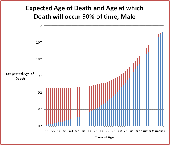
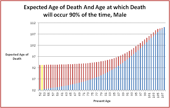
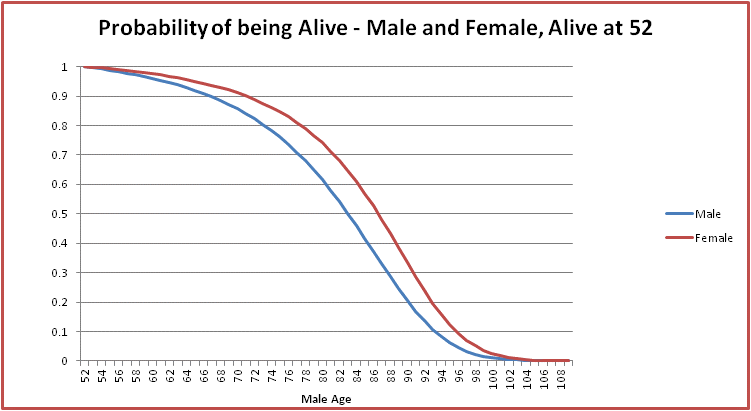
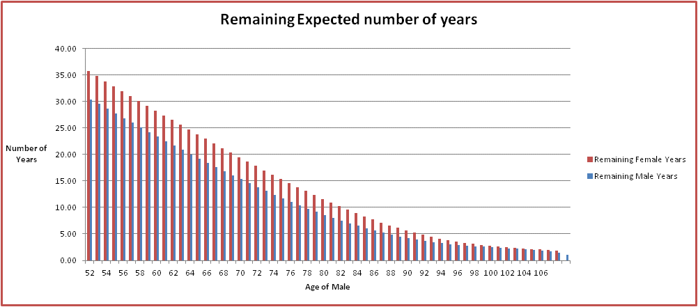
There are many planners around the web which will give you an indication of how long you and your spouse will live and this can be a useful input into Superannuation planners.

According to this one, http://www.mylongevity.com.au/, I will live to 84. Another one told me I will live to 86.

This diagram in the nytimes is quite interesting as it gives you an idea of the volatility of the markets:

http://www.nytimes.com/interactive/2011/01/02/business/20110102-metrics-graphic.html?_r=3&

Also on numerous sites is the 4% rule. According to this rule, you can retire if your annual spending will be no more than 4% of your financial assets. So if you want to spend $50K per year, you will need $1.25M. Note that there is no length of retirement in this calculation. This rule assumes you can make 4% + inflation on your assets through investments, so that you never lose your capital.

Although I found all these planners and tools to be useful, I found that that they did not provide all of the information that I require to plan my retirement. In particular, the following is missing:

• Functionality – The planners do not cater for things such as asset sales, changes in spending patterns as we age, existing on cash prior to 60 etc.
• Sensitivity Analysis – How are my retirement plans impacted by varying some of the key assumptions – e.g. the age of stopping working, the age of spending all assets, the returns from Super etc.
• Products – The planners do not allow me to look at how I would fare using different products (e.g. lifetime annuity versus account based pension).
• Risk – The planners do not tell me how my plans are impacted by variable super returns, or how my plans would have fared in various historical scenarios.
• Baseline Plans – There is no ability to create a baseline plan and compare progress against the plan.

For these reasons, I have developed my own set of tools. While these tools presently consist of spreadsheets, if I have time available I will endeavor to put these online.

Australian Superannuation and Age Pension Rules

In the following sections, I have worked out how we will fare in retirement under various scenarios. I have strongly leveraged the information in the “Australian Superannuation and Age Pension Rules” post in this blog. It contains the Government rules that are applicable to early retirement. In order to fully understand our strategy and the various scenarios, you will need to familiarize yourself with these rules. These rules should also be useful for your own planning.

Our Retirement Strategy

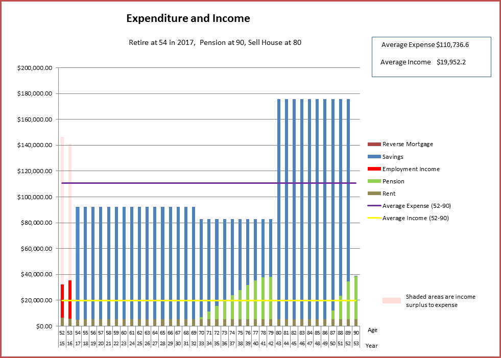
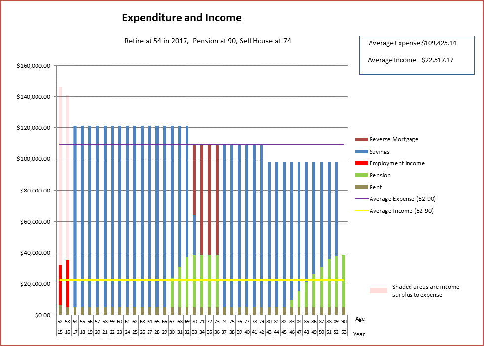
We are planning to use cash to finance our living expenses until it runs out, then use superannuation, possibly supplemented with the Age pension. Before I hit 65 (about 13 years away), we will sell our house and put the funds in Super. We will take advantage of the “Bring Forward” superannuation rule to put the proceeds of the house sale into Super in one year. We will then move to either our investment house or our retirement house near the sea. We do not plan to sell our investment house.

My Calculations

In this section I work out the funds we can expect to be available to us each year, assuming we retire in early 2015 and we use the retirement strategy above. I have used Excel and Excel VB macros and the rules in the “Australian Super and Age Pension” post to do this. The Excel “solver” function is the critical function that I have used, as a complicated equation with boundary conditions is required to be solved.

For the purposes of the calculations, I have assumed that:

• We will spend 10% less per year when we hit 70, and another 10% less when we hit 80. The studies that I have read indicate that this is a reasonable, if conservative, assumption due to lower mobility when you age (and even taking into account higher medical bills). There is an interesting paper on this here.
• I will live to my 90^th birthday and at this point we will no longer have any Super. After this if we are still alive, our only source of income will be the Age pension and rent.
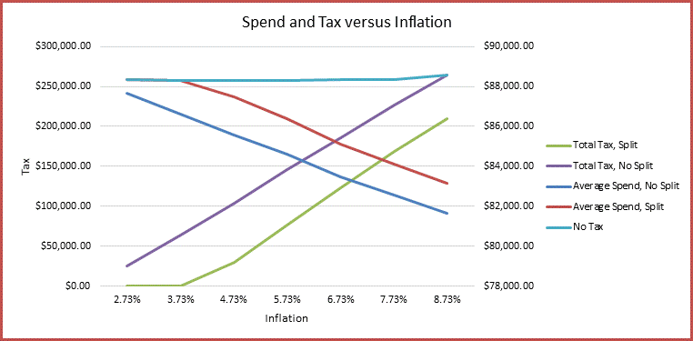
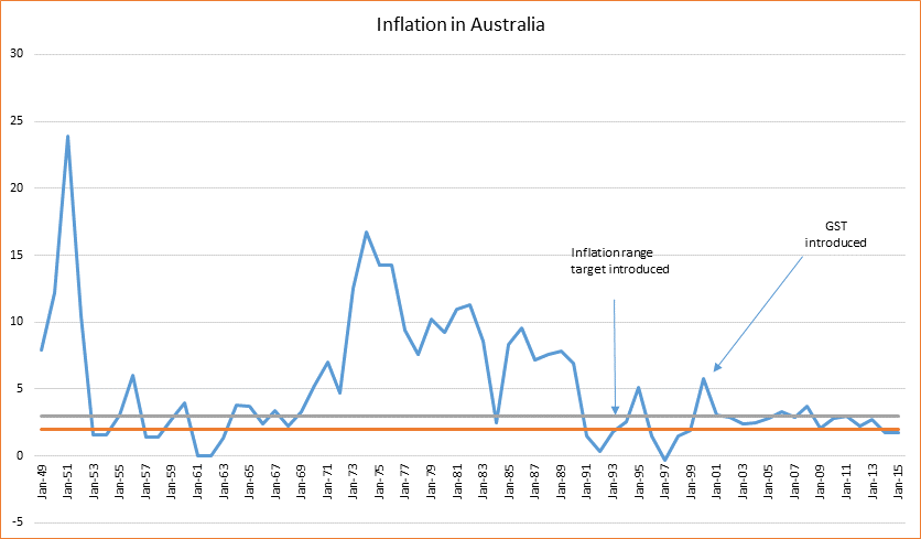
• Inflation will run at about 2.73% per year. This is the average since 2004. This assumption will obviously almost certainly not hold true, but hopefully Super returns will compensate in the event of higher inflation.
• Rules relating to the Age pension don’t change. Again, this is unlikely to be the case. But I have based the calculations on existing rules as there is nothing else available and the rules when I retire will probably be similar to the existing rules. Some people have suggested that, in view of the uncertainty about Age pensions in the future, it may be best to model based on the Age pension being unavailable. I have done this modelling; you can see it here.
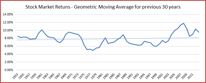
• Superannuation returns, nett of all fees, are 5.5%/year nominal, i.e. not adjusted for inflation. This is an equivalent of about 2.8% real return. Note that Australian Super balanced fund has averaged 8.69% per year since 2004, or about 6% real return, and this includes the GFC! (nominal – For each year from 2004 I have subtracted the inflation rate for that year and added in 2.73%, then averaged to get the 8.69%).
• On my 60^th birthday I will move our Superannuation funds into an account based pension. As a result our Super returns will be improved due to lack of tax. I will assume that my Super fund was paying 8% in tax. So that means that after 60, returns on my pension will not be 5.5% but 5.5/.92 = 6.0%, or about a 3.3% real return.
• We only spend $40K during 2015 and earn $20K (working for some of 2015) from employment and $5K from rent. Subsequent years involve spending the amount indicated in the graphs below.
• We sell our house just before my 64^th birthday. This will leave a year’s buffer to ensure that we can move the funds into Super in time.
• Cash rate is 3.2%
• We continue to receive rental income from our investment property while we are alive.
• The rate of house appreciation is 2.83% (the average for my house over the last 10 years).
• We do not borrow any money or take out reverse mortgages.
• To work out our spend per year, we always maintain the same real value of spend year on year given the available assets over a particular time period and also given any planned changes in spending, with the goal of minimizing the available superannuation on my 90^th birthday over the long run.

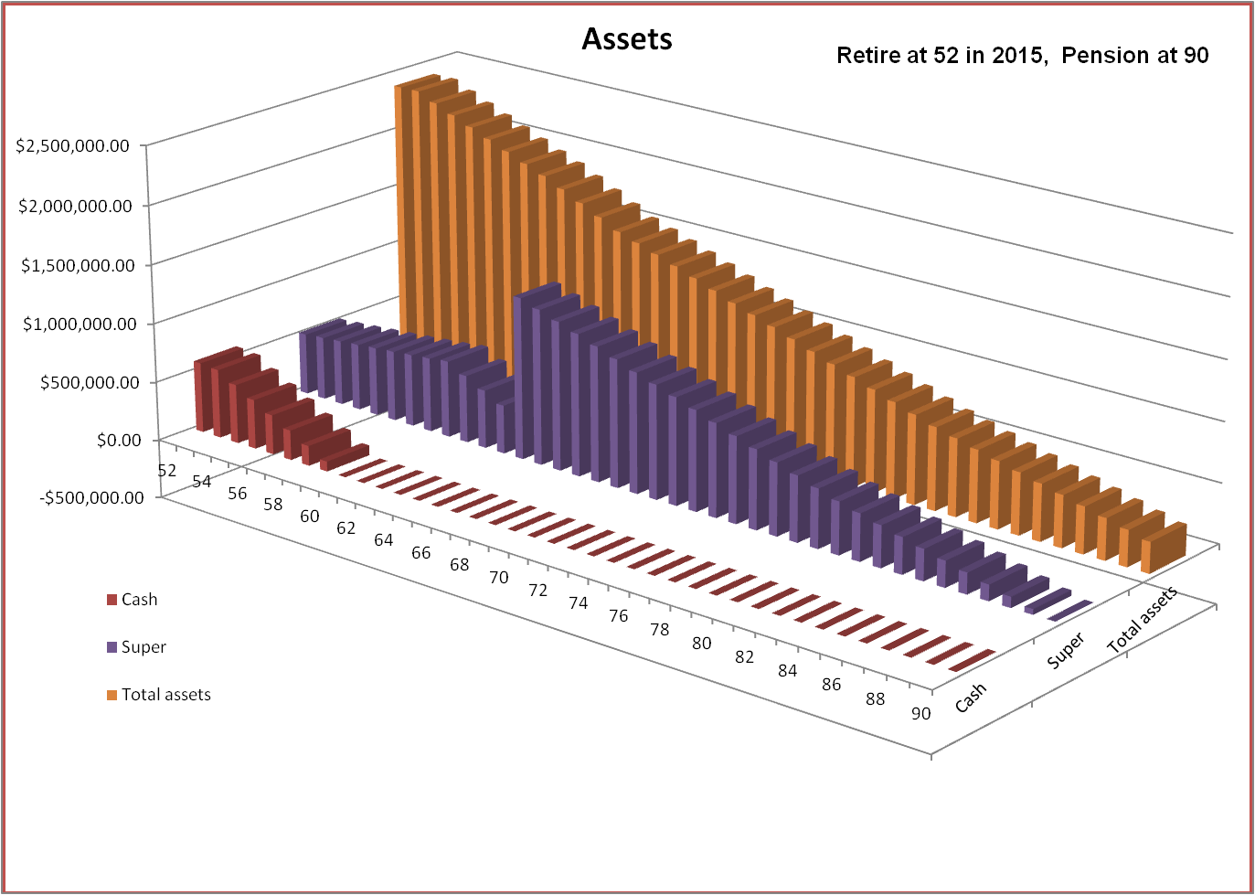
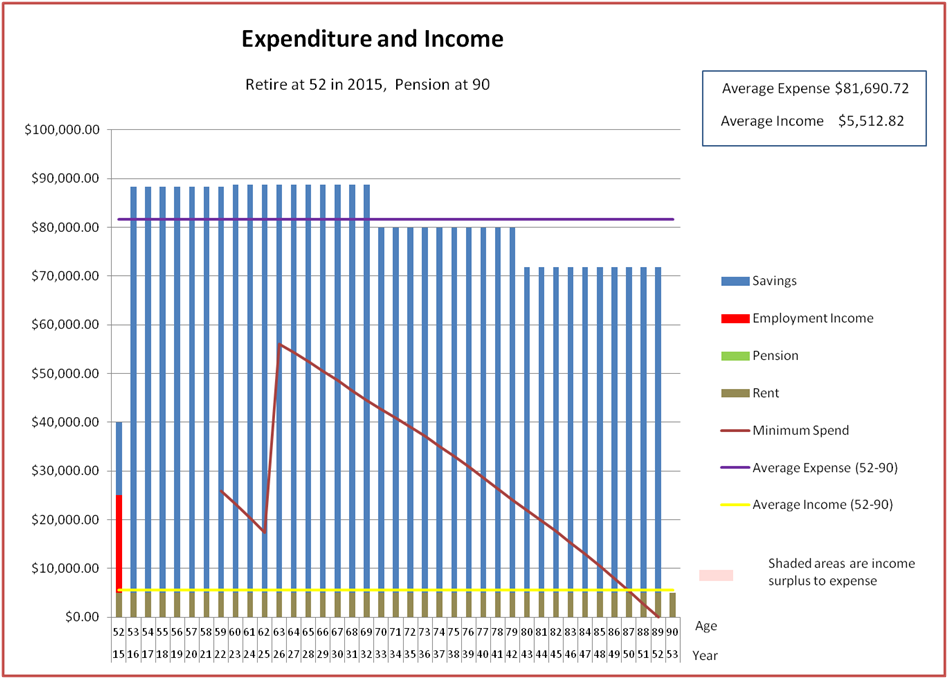
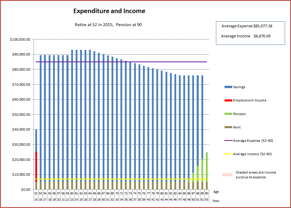
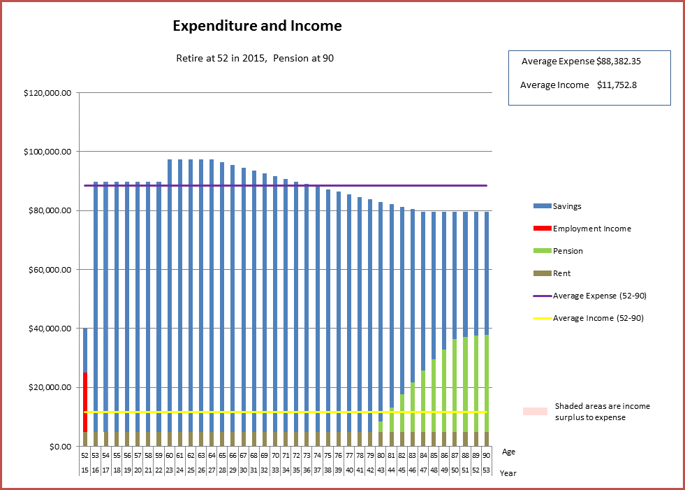
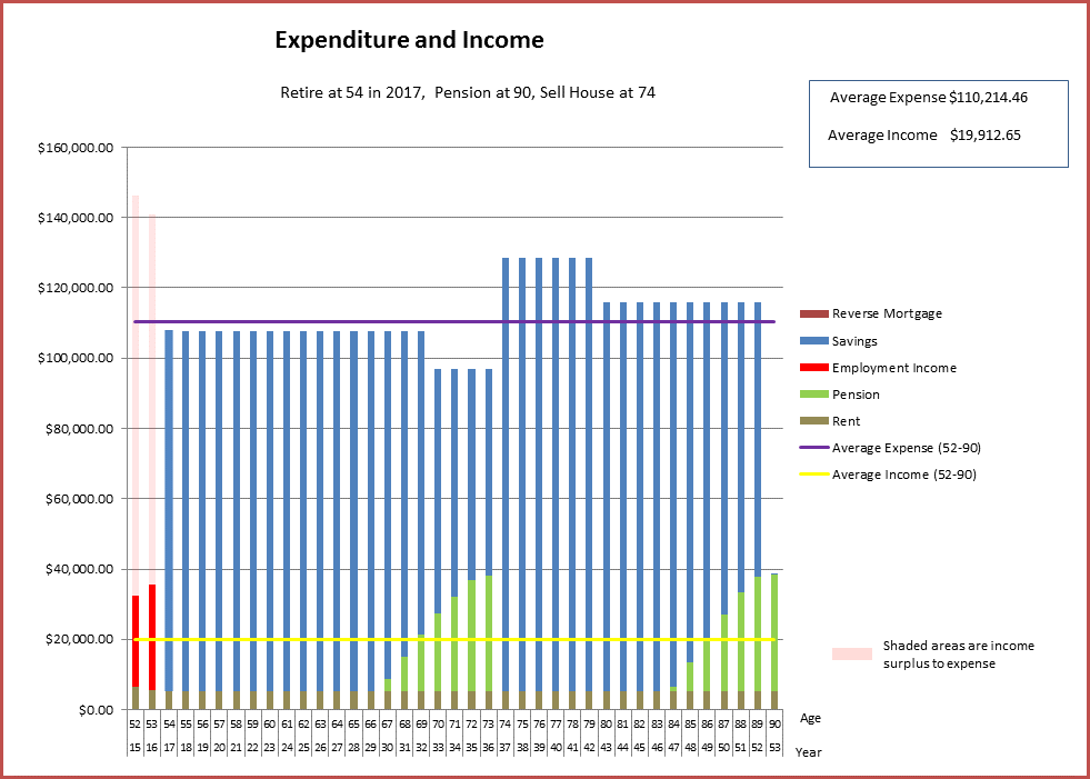
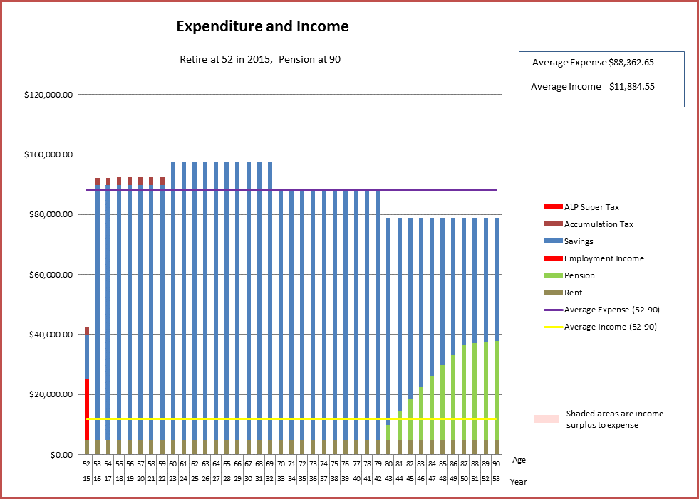
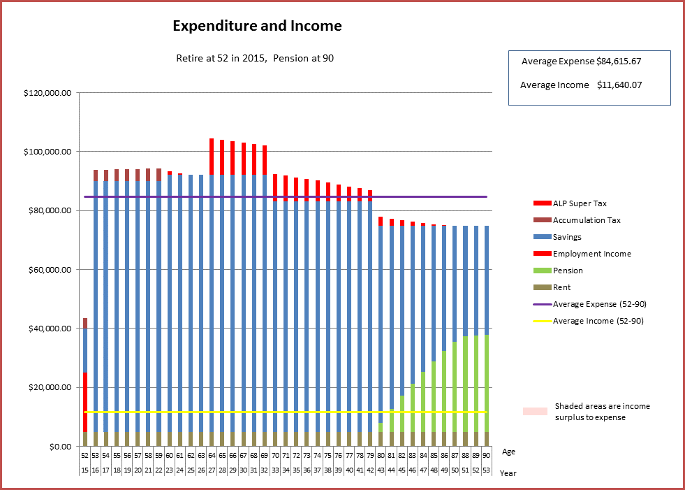
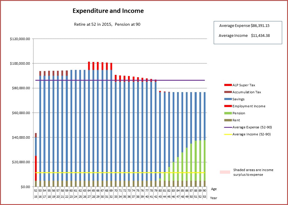
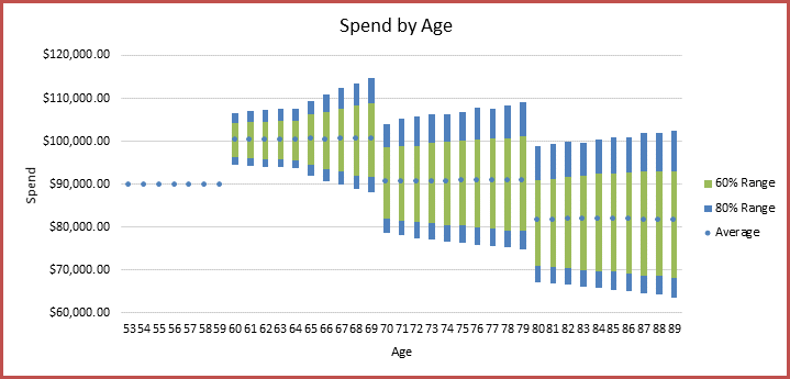
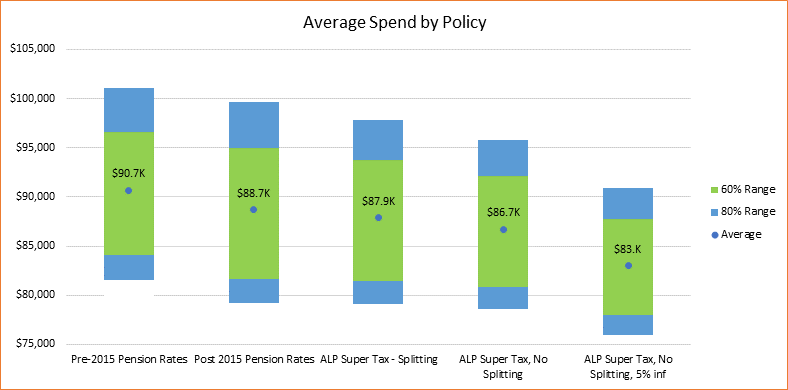
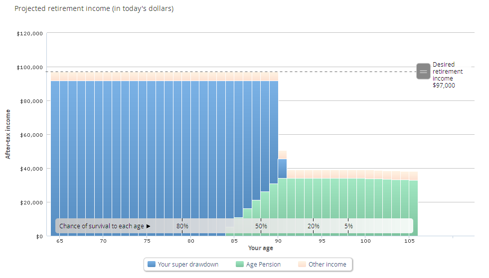
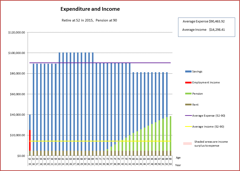
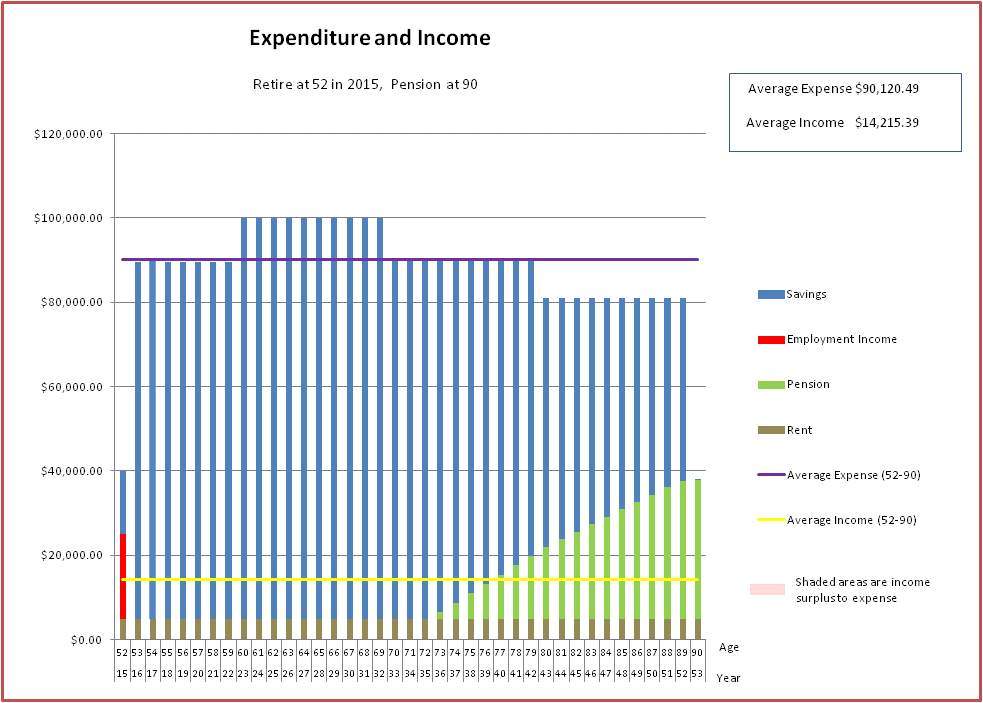
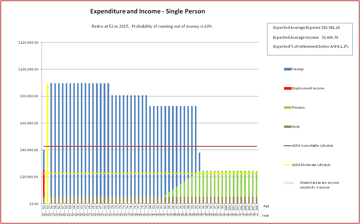
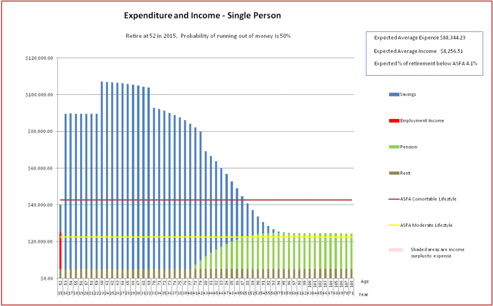
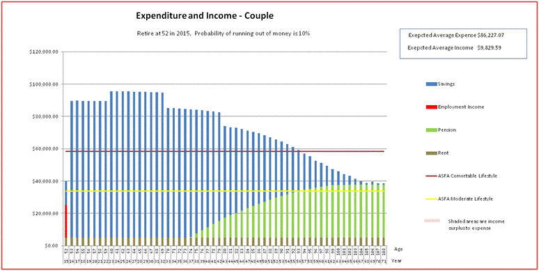
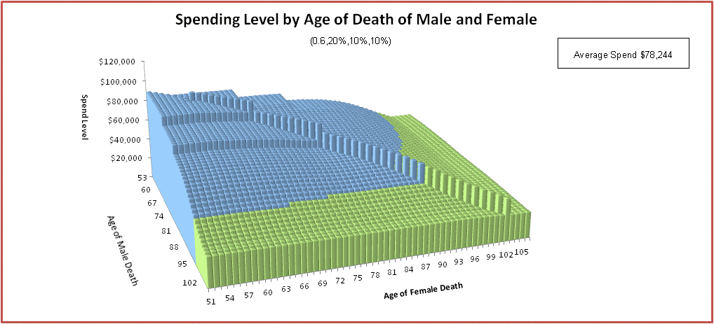
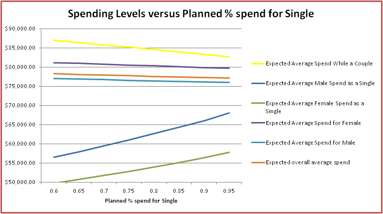
The graph below is the result. It is in real 2015 dollars. You can see the age pension kicking in at around 74. The spend prior to 60 is less than after 60 due to limited cash assets prior to 60. Average expense per year is about $87K. I’ve also included the minimum spend required by the account based pension. You can see that it is not a factor here.

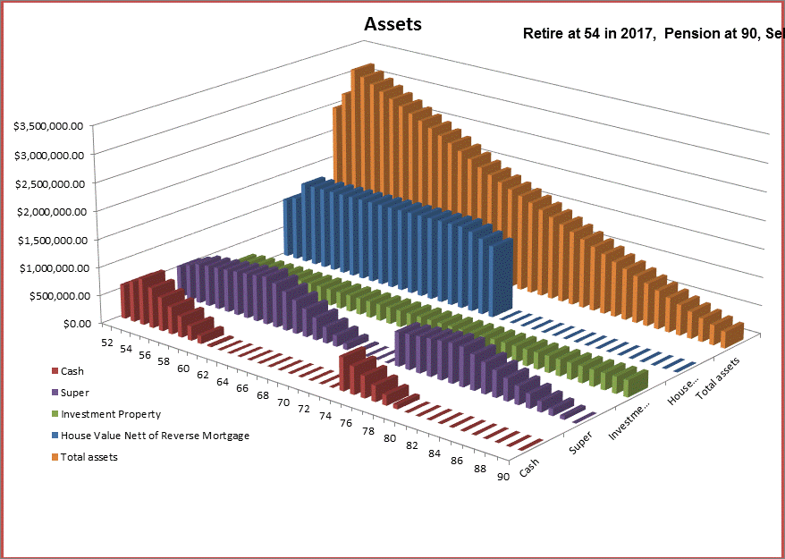
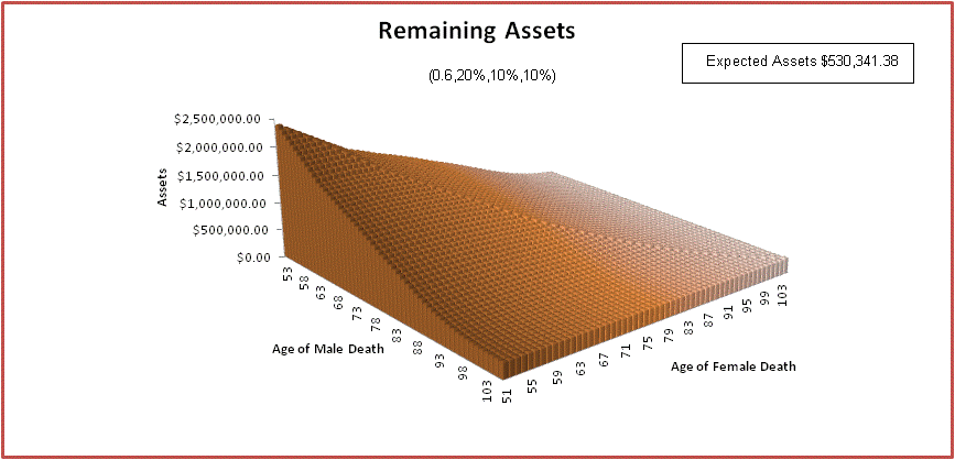
And here are the assets. You can see the super going to zero in the last year that we are planning to supplement the pension with Super. Total assets at 90 isn’t zero because we are planning to keep our investment property.

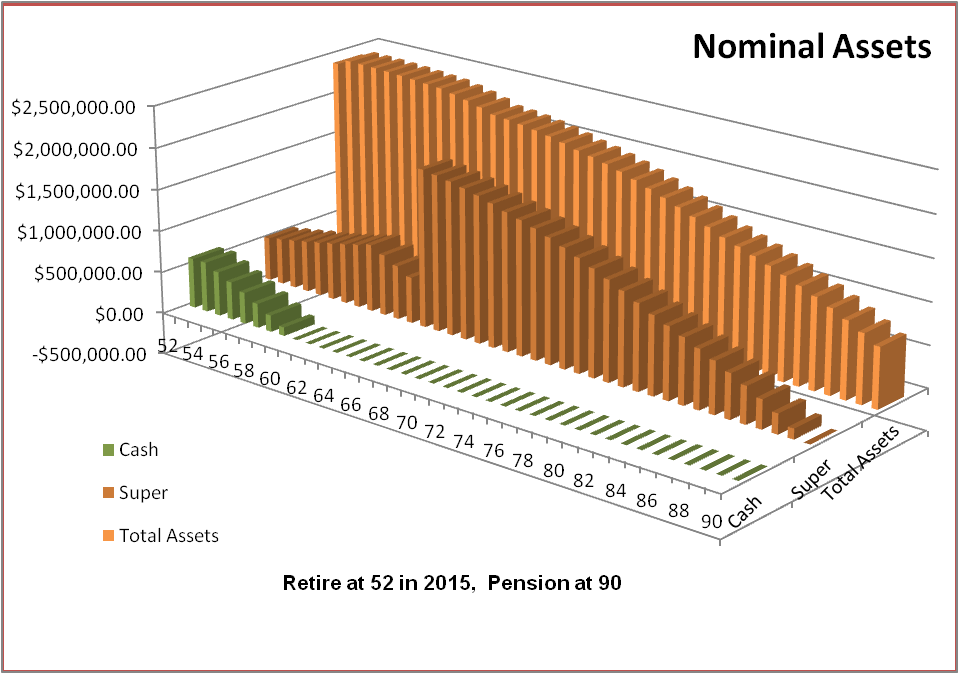
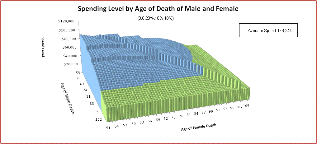
Here is the graph in nominal dollars (that is, not adjusted for inflation):

For those who are interested in such things, the way I have made the calculations is described at the end of this post in end notes.

Sanity Checks

In order to check the results of the calculations are reasonable, I did some sanity checking by looking at the results of some online calculators and compared them with the results of my model. Due to the difficulty of some calculators with handling living on cash prior to accessing Super, and with asset sales, I started the calculations at 64. Also, most calculators can’t handle changes in spending profile over time, so I removed the reductions in spending at 70 and 80. I kept the investment property and the investment income as most (but not all!) calculators are able to handle this. If I do this, my model shows the Super level at 64 to be $1,409,596 and average spend to be $87,826 (both in 2015 dollars). If I enter these details (Super level, investment property, investment income) into the online calculators, as well as trying to make the inflation (2.73%), Super return levels (6.0%), fees (0%) and age when Super will last until (90) as close as possible to my model, I get the results summarized in the diagram below:

RNU is this website. Interestingly the ASIC site provides a much lower spend than most other sites.The above diagram shows that the results from my model are reasonable, with my site being very close to the average of all sites.

I also computed the spend using the calculator default inflation, Super return, fees and age at which Super lasts until.  This results in an average spend increase of about $2000.

More details below:

Note that the average real default return (3.29%) is very close to my assumed real return (3.25%).

Which calculator did I like best? Actually the VicSuper one was quite good as it allows you to enter the investment property and investment income, and also provides a band of outcomes, depending on the riskiness of the investment. It is a “type II” calculator, meaning that you have to fiddle with the spending levels so that you get your funds lasting until 90. It doesn’t allow you to enter the Super returns level and only allows you to specify risk levels of the fund, but this is only a minor inconvenience.

Sensitivity Analysis

Having established that the results from my model are similar to those provided from other planning sites, I will now use the model to perform some sensitivity analysis around some of the key assumptions.

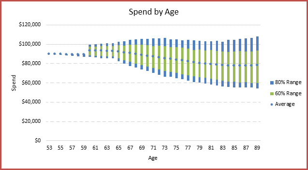
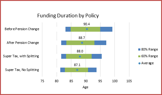
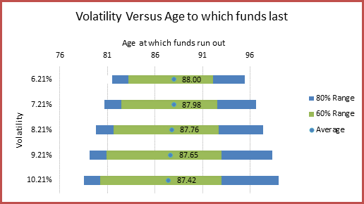
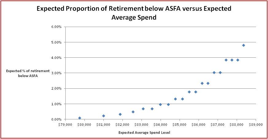
Here I worked out the sensitivity of the expense per year to Superannuation returns. Basically very sensitive. Later in the blog I look at how expense per year would have fared in some real historical situations. The super return rate I have used as part of my assumptions is highlighted in red.

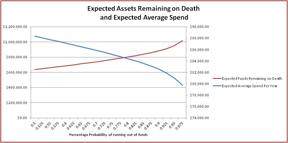
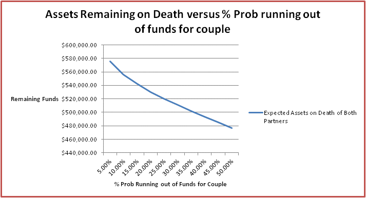
And here is the sensitivity to when we decide we will go on the age pension (i.e. when we are planning to have no super left). Not really too sensitive. I think 90 would be an OK age to plan for. The below diagram is saying that if we plan to spend all our money prior to 75, for example, we can expect a spend per year of just under $120K (rather than $87K). However after 75, we will be living on the age pension.

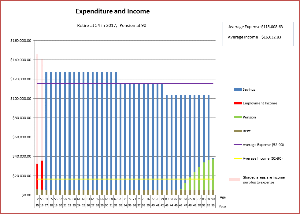
Then I worked out how sensitive the expense per year is to working additional years, assuming an annual expense of $40K per year while working, while still spending only $40k during the first year after stopping work. My average expense per year goes up by about $4.5K per year for every additional year that I work. The average expense per year goes up a bit more if I just consider the time after retiring.

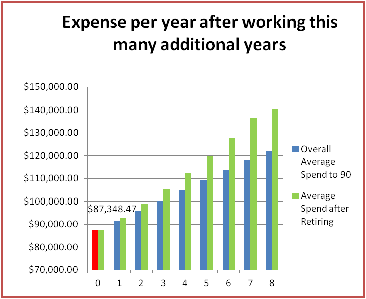
Because the effect of working additional years is of particular interest to those considering early retirement, I have provided a summary of the details for each additional year of retiring here:

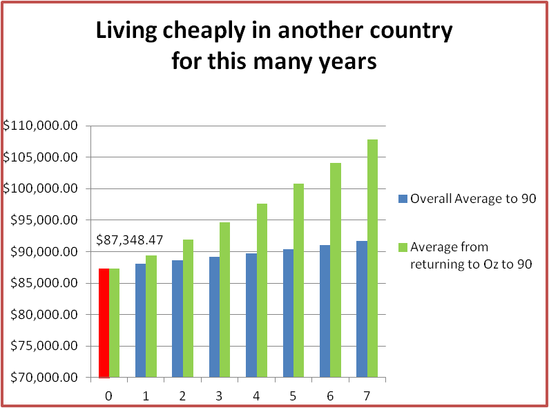
Lastly I looked at living in a cheap country for a number of years prior to fully retiring in Australia. Living in somewhere like Chiang Mai could be interesting. I assumed that we can live on $20K per year (+ rent from our property in Australia). You can see the average expense per year after we return doesn’t really go up much as a consequence. Note the rule regarding CGT on your home is applicable here.

Market Exposure and Risk

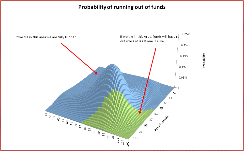
The next thing I did was to work out how risky this strategy is and how exposed to the market we are based on past performance of the market. The firecalc tool mentioned above is quite handy in this regard. However, I have added in support for Australian conditions, and also assumed that when our capital is reduced, we will also reduce our spending rather than spending the same fixed amount every year.

The idea is that I assume we retired at the start of a year between 1923 and 2012, and then worked out how much we would have available to spend that year based on the the assumption that the market would perform at 5.5% (pre 60) and 6.0% (after 60) for the remaining years with an inflation rate of 2.7% (just as I did at the start of the post). Next I look at the actual return for that year, work out the actual Super available at the end of year based on this return, subtract the amount spent during the year, and then repeat the calculation of how much I have to spend, again assuming the same return and inflation. I do this until I am 89. Note that the assumption of a 5.5/6.0% return only impacts the amount of money spent during a year, and does not impact on the actual performance of Super. The actual performance is taken from historic market returns. Also note that I am using raw market performance which is not moderated as a “balanced” superannuation fund would be.

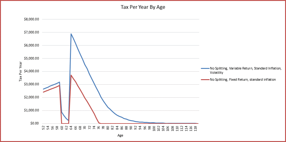
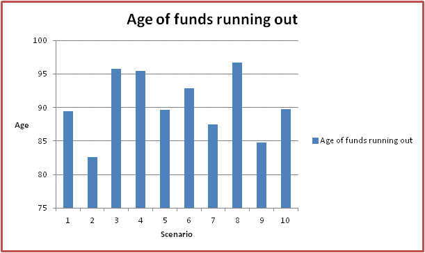
Anyway, If I do these calculations for each of the years between 1923 and 2012, it turns out that the worst year to retire was 1969 with an average expense per year of about $83K and the best year to retire was 1978 (getting the bull run of the 1990s when my house was sold) with an average of about $148k. The average expense per year across all years is about $105k.

I obtained historical information on the Australian market performance from here:

http://www.wrenadvisers.com.au/downloads/ (yxaoi.xls)

(I think there should be a better source than this, but could not find one).

I also obtained historical information on inflation in Australia from here:

http://www.rba.gov.au/inflation/measures-cpi.html

And also estimates of Dividends from here:

http://www.macrobusiness.com.au/2011/06/relying-on-stock-market-averages

Here is a summary of the extracted historical information (real returns):

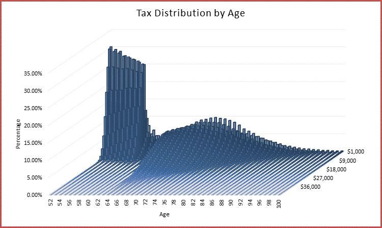
Here is the average expense per year graph mapped out against retirement year. Excel took about 30 minutes to produce this graph due to all the Solver functions required!

Note that there is a cap on the minimum spend – that is because before 60 there is a cap on the spend per year due to the limited assets prior to 60. This spend per year prior to 60 can go down however, if Super performs poorly.

You can see from the above graph that in most years the average expense per year computed using actual market returns is a lot better than that computed using the assumed returns of 5.5/6.0% (i.e. 87k). In 9% of the years it is worse, but almost all of these years are recent because recent years assume a 5.5/6.0% return for most of the subsequent years (as there is no historical data). The  only other that is not recent is in 1961.

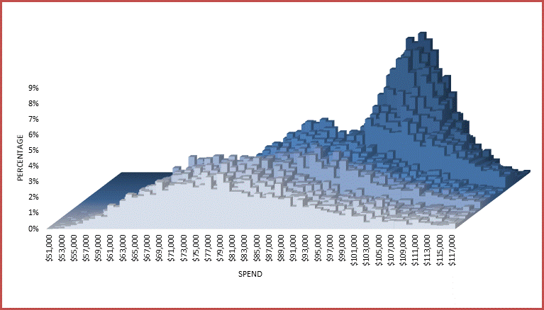
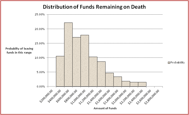
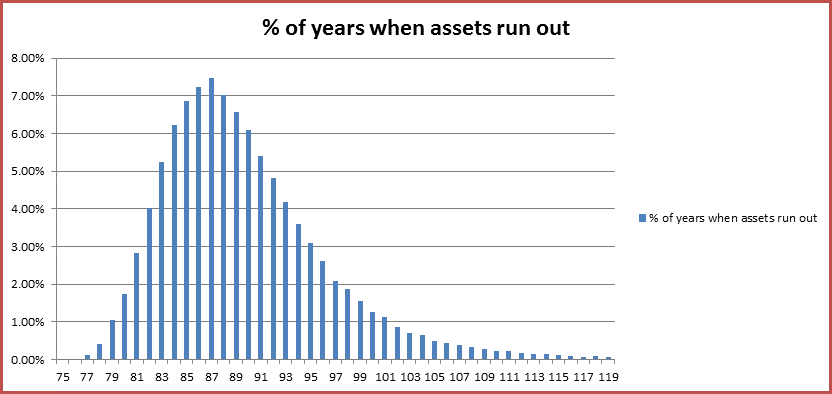
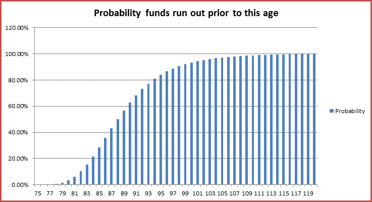
Here is a graph showing the distribution of average expense per year:

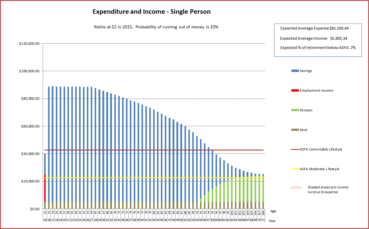
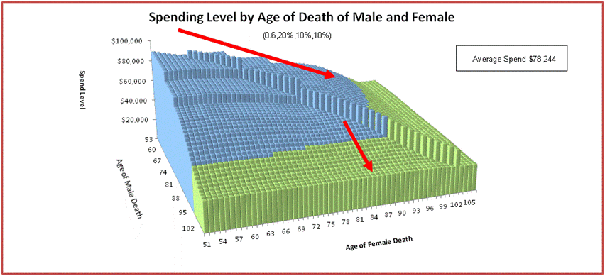
The below graph illustrates the expense per year for commencing retirement in the worst year (1969). Note the age pension cutting in a 67. Also note that in some years we only have about $67k to spend. The average of all the bars in this graph is about $83K, the value that corresponds to the 1969 bar in the expense per year graph above.

And here are the assets for commencing retirement in the worst year. Note also that the actual graph is nothing like the smooth graph assuming the constant return of 5.5/6.0% shown earlier in the blog.

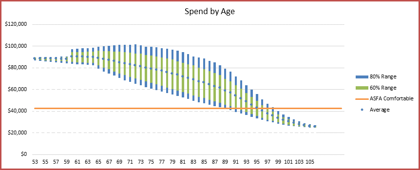
And here is the expense per year for the best year for commencing retirement (1978):

Note that the expense per year us flat prior to 60. This is because we are living on cash during this period prior to getting access to Super and the amount of cash is fixed. Also, the expense per year is flat after 2013. This is because we are now using the standard 5.5/6.0% rates (i.e. I have no market data after this).

And the assets for the best year:

Some people have commented that the reactive type of spending plan proposed here may not always be realistic as people often have fixed commitments which cannot be adjusted every year (e.g. golf club memberships etc.). However, at least in my case, our only high expense items we are planning is traveling, and we can easily cut back on this. I think cutting back in the event that Superannuation assets are reduced is a good idea. It prevents you from running out of money.

Lifetime Annuities

Most Australians either take out a lump sum, or purchase an Account based pension in their retirement. However there is another option, the lifetime (or fixed term) annuity. These types of products offer the advantage of income certainty, and also eliminate the risk of running out of money. The provider takes the risk.

How do strategies based on commercial lifetime annuity offerings stack up against my proposed strategy?

Using a popular Australian lifetime annuity product,  I have chosen the income stream with full inflation protection starting from 65. In early 2015, this provides $3202 per annum for each $100,000 investment (for a male) until you die. It also provides a 100% income withdrawal guarantee, meaning that if I wish to withdraw the capital after 15 years, I get 100% of the capital back (unadjusted for inflation). 65 is the earliest published age at which rates are available, so I will assume that we will exist on the Account Based Pension to this age using the original plan, and then at 65 withdraw all the funds, and invest in the annuity. I will then compare the annuity with the account based pension after 65.

According to my model at 65 we will have $1,313,701 in Super in 2015 dollars. If I purchase the annuity with this asset at this age, then the annual income provided by the annuity after 65 would be $42,064. If I use half the money to pay for an annuity for my wife and half for an annuity for myself, and for the purpose of this exercise assume my wife is the same age as I am (as the company offering the annuity does not publish age-by-age annuity incomes),  the amount would be $41,623. The amount is slightly less as females have a longer life expectancy than males. Note that a jointly owned annuity may give a better return, but the rates for this type of annuity are not available on the web site. Adding in rent received ($5,000) I can then work out the spend available each year using the annuity approach. To do this, I have used this section in Australian Super and Pension rules post. Note that:

• We cannot roll-over our Super Money to pay for the annuity as this is only possible if we have “unrestricted non-preserved funds”. I do have some of these type of funds, but only about $90K. Instead, we would have to take our Super out as a lump sum, and then purchase the annuity with these funds.
• As we will not be rolling over Super, we will have to pay PAYG tax on the income received. As the income received would only be about $23K each, and the “Deductible Amount” is higher than this (at least initially) and we also get an offset amount using SAPTO from Age Pension retirement age, there will be no tax to pay. If you had a higher income from the annuity, income tax may be a consideration.
• The Age Pension assets test uses the initial purchase prices of the annuities, less the “Deductible Amounts” accumulated to date as explained here.
• The Age Pension income test does not use deeming of the asset value. It uses the income from the annuity, less the deductible amount. As it appears that the deductible amount is not inflation adjusted, that means the income test becomes more important as you age.

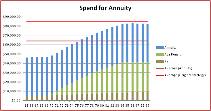
Here is the graph showing the spend for the annuity:

Note that:

• The average spend for the annuity, assuming we both live to 90 exactly, is $63,800, while the estimated average spend for the Account Based Pension is $85,300. Or the annuity average spend is about 75% of the Account Based Pension amount.
• Barring changes to Government rules, the lifetime annuity amount of $63,800 is fixed and will not vary, while the Account-based Pension amount is variable and subject to market returns.
• The spending pattern is counter to the spending pattern that most people would like. That is most people would like to spend more in their earlier years and less in the later years.
• The Age pension starts to decline as you age, because the incomes test becomes more effective. The “Deductible amount” is not inflation adjusted so it becomes less effective in reducing the income from the annuity and therefore reducing the reduction to the Age Pension due to the incomes test.

If we live beyond 90, the lifetime annuity becomes more attractive, because with the Account Based Pension we will be living on the Age Pension (+rent) only, whereas with the lifetime annuity we will continue to be funded by the annuity. Still, the average income from the annuity only exceeds the estimated average income from the account based pension if we both live to 106.

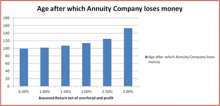
The other way to look at the Lifetime annuity is to work out the present value of the payments from the provider assuming we live to certain ages. The graph below provides information on the age to which we would both need to live in order for the provider to lose money, assuming various discount rates..

An Alternate Strategy

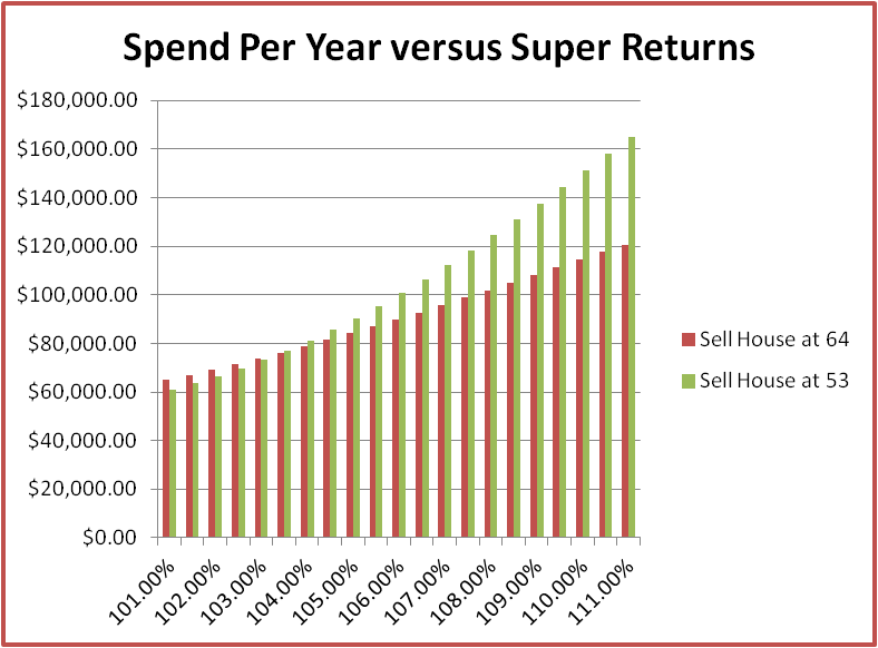
One of my relatives has decided to sell up in Australia and go and live in Thailand for an indefinite period. Which makes me think about doing something similar. Perhaps selling up our house and maybe traveling for some time. Surely selling up and putting all the funds into Super would amplify our savings and give us a much higher spend per year? As a safety net, I have assumed that we will not be getting rent from our investment property once we have sold up (as we might live there). I also assume we will fully retire at 65 by living at our final destination.

Well, I did these calculations and got the graph below:

Surprisingly, there is not that much difference. If we decided to sell up at 53 and go vagabonding  we would have about an extra $9K per year.

However one impact of selling your house early and putting funds into Super is that you are much more exposed to the market. If the market does well, you will have significantly higher spend. For example, if returns are 9% you will have a $137K spend if you sell your house at 53, while only $108K if you sell it at 64 with the same returns. The graph below shows the expense per year assuming a house sale at 53 versus a house sale at 64. Note that if the market performs poorly, say 1%, then selling your house early will put you in a worse position ($61K versus $65K), but not significantly worse. There is mostly upside assuming very poor returns (e.g. typical of the 70s) do not occur.

What if there was no Age pension

Some people say that you should plan as if there was no age pension. Well, if I do this, I get the graph below:

Actually not too much of a difference..

What could go Wrong?

Could we experience another decade like the 70s? Yes, I think we could. Maybe more than one decade. But we could also experience some boom decades as well. No-one really knows.

On the negative side, over the next few years we have the following happening:

• The ratio of workers to retirees is getting smaller as the baby boomers retire. Less workers to produce goods and services and more non workers to consume them may mean that goods and services (especially services that can’t be outsourced to other countries) will become more expensive.

• The world is running out of fossil fuels. Goods and services may become more expensive as more expensive substitute fuels are used instead of cheap fossil fuels.

• The world is heating up and we may need to use more expensive fuels to compensate. Or agriculture could suffer in a warmer world.

• As more workers retire, the Australian government may decide to change the pension and Superannuation rules in order to reduce the social welfare bill.

On the positive side we have:

• The developing world is contributing to the world economy more and more. Things are getting cheaper as large quantities of cheap labour enter the world economy. These workers are also getting more productive as they adopt first world technology and become more educated.

• The world is becoming more connected and innovation is occurring more quickly. In addition the developing world is starting to contribute to innovation and R&D as education levels increase.

• Australian worker productivity is expected to increase over the coming years. An increase in productivity will mitigate  against declining overall production caused by declining worker ratios.

All of these may effect the amount of funds available in retirement.

Conclusions

So, what are my conclusions?

• There are various tools on the Internet which help you work out when you can retire, however I have found that they are, in general not adequate to plan your retirement. They do not cater for changing spending patterns, asset sales, etc. The determined pending retiree (aka yours truly) can develop more suitable tools, but this is time consuming and requires mathematical and financial skills.
• Sensitivity analysis can be used to understand how key variables affect the average spend you can expect in your retirement. This analysis can help you make decisions such as how long to keep on working, the age at which you should plan to live on the Age Pension only, the sensibleness of spending some time in a low cost country, etc.
• Historic market performance data can be used to generate information on how you would have fared in your retirement had you retired in earlier years. This information can be used as an indication of how you are likely to fare in your actual retirement.
• It is possible to compare spending levels between a lifetime annuity approach versus an account based pension approach. Initial analysis indicates lifetime annuities do not provide good value, and should only be considered if you put a very high premium on income security or expect to live a very long time.
• It is possible  to work out your spend levels assuming there is no Age Pension. This information can be handy, especially if you are concerned that the government may be cutting back on the Age Pension soon.
• If you decide to sell your house early and invest in Super, then you can expect higher spend, especially if the market does well. But of course this may come at a cost e.g. through less salubrious accommodation.
• The future is uncertain and there are various factors which are working towards making a retirement more comfortable, and others working in the opposite direction. We will have to see how things pan out.

And what am I going to do? Probably work a few more years. I work in IT, and it seems it is not that easy to get work once you get to my age, although I haven’t had any problems to date. But it’s nice to know that we should be able to retire if we want to :).

End Notes

In this section I will provide information on how I have worked out the numbers behind the graphs by describing the formulas used to calculate funds in each year. It’s actually several big complex non-linear equations that need to be solved. Fortunately Excel “solver” can do just this.

A note about terminology: When I refer to “year i” below, this is the year that commences on my i^th birthday.

Also, while these formula are particular to my situation, they can easily be generalized to cater for the asset sales and purchases typical in retirement.

Constants

B_D = Bank Cash Rate of Interest= 3.2%; This is the daily rate. B_Y is the yearly rate and B_C is the continuous rate.

I_Y = Inflation = 2.73%;This is a yearly rate. I_C is the continuous rate.

H = Rate of property appreciation = 2.83%; This is a yearly rate.

Variables

N = Age of selling house. M = Age of purchasing account based pension.

R = Age of Retiring. A = Age we are planning to only have rent supplementing Age pension.

R_i = Rate of Increase of Super during year i;. R_i = 5.5% for i < M, R_i = 6.0% for i >= M.

C_i = Cash at beginning of year i; I_i = Income in year i (employment + age pension);

S_i = Value of Super at beginning of year i;

P_i = Value of primary residence at beginning of year i;  T_i = Value of investment property at beginning of year i;

D_i = Value of rent received during year i;

W_i = Estimated tax free income while working during year i.

X_i = Estimated expense while working during year i.

U = Estimated expense in first year after stopping working in 2015 dollars

V = Estimated Residual income in the year after stopping working in year 2015 dollars. i.e. any income earned in this year.

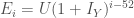
E_i = Expenditure during year i in year I dollars. E_i is of interest as these are used to plot the graphs.

Initial Conditions

C₅₂ = $595,000; S₅₂ = $520,000; P₅₂ = $1,029,000; T₅₂ = $250,000; D₅₂ = $5000;

R = 52, N = 64, M= 60, A = 90,

if R > 52 then W₅₂ = $120,000 else W₅₂ = 0

if R > 52 then X₅₂ = $40,000 else X₅₂ = 0

U = $40,000, V = $20,000,

What we are trying to solve for

We are looking for the values of:

E_R+1 that minimizes S_A.

Subject to:

S_A > 0,

> 0

S_N – P_N > 0

That is, we want to work out the expense in year R+1 (the year after retiring) that minimizes the amount of funds we have left at 90, subject to:

• Funds left at 90 must be greater than zero.
• The year before taking out the account based pension, our Cash and income must be more than our expenses. That is, we need to make sure that our expense levels prior to getting access to the account based pension don’t cause us to run out of money.
• The amount of Super left at the end of the year before selling the house must be positive. That is, we need to make sure that our expense levels prior to getting access to the additional fund from selling the house don’t cause us to run out of Super.

We also want to find E_M that minimizes S_A.

Subject to:

S_A > 0,

S_N – P_N > 0

That is, we want to work out the expense in year M (the year during which we start on the account based pension) that minimizes the amount of funds we have left at 90, subject to:

• Funds left at 90 must be greater than zero.
• The amount of Super left at the end of the year before selling the house must be positive

and lastly

E_N that minimizes S_A.

Subject to:

S_A > 0.

That is, we want to work out the expense in year N (the year during which we have access to the funds from the house sale) that minimizes the amount of funds we have left at 90, subject to:

• The amount of Super left at the end of the year before selling the house must be positive.

These Solvers need to be done in the order in which the events causing the assets to change occur (e.g. if I sell my house before accessing Super, then this one should be done first, and the boundary conditions will also need to change to reflect this).

Formula

First the easy ones:

(i)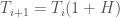     

The investment property appreciates every year.

(ii)       if i < N then 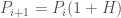else 

The primary residence appreciates every year until it is sold when I am 64.

(iii)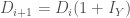     

Rent from investment property increases with inflation.

(iv)      (a) Except for i+1 = M, N and R+1, for  i >= R,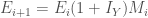 
where M₆₉=0.9; M₇₉=0.9 and M_i=1 for all other i. E_R+1, E_P and E_N are derived from solver equations described above.

That is, expenditure goes up with inflation each year, but is reduced by 10% at 70, and another 10% at 80.

           (b) If R > 52 then for i < R, E_i = X_i

(v)      For , 

Year after retiring, I spend U.

(vi)      If i < R then else

(vii)      If i < R then  else

(viii)     if i = R then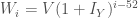

Working income and expenses increases with inflation, and become zero when I retire.

(ix)      For i < 67, I_i = W_i

Income is employment income prior to 67.

Now for the more complicated ones. Here is the formula for Cash at beginning of year i+1:

(x)     if 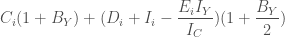  < 0 then C_i+1 = 0

         else

where

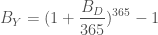
and

This says that if the cash at beginning of year i +  rent received during year i + Income received during year i + interest on cash during year i is less the amount spent during year i, then the cash in year i+1 is zero. Otherwise it is the cash at beginning of year i +  rent received during year i + Income received during year i + interest on cash during year i less the amount spent during year i. Note that in the year that expense exceeds cash that is non-zero, the excess Cash is added to Super for that year only.

And here is the formula for Super at the beginning of year i+1:

(xi)     if > 0 then

        else

This says that if expenses is less than cash + other sources of income for the year, then Super just increases at the super return rate. This is because cash will be used to fund expenses while it is available. Otherwise to work out the new super value we need to deduct expenses and add in any income and then multiply by the Super return rate. Note that if we cannot fund expenses from Cash then Cash will be zero for all years except the first year where this occurs. So, I have added in Cash to working out the new value of Super; this will be zero for all years except the first year, where I have assumed that the Cash will be added to the Super pot.  I’ve also added in the value of the house when I sell it.

Now for the most complicated one. Working out the age pension.

For this one we have the following variables:

P_ULi = If your assets are above this at the start of year i, then there is no part pension.

P_LLi = If your assets are below this at the start of year i, then you get the full pension.

P_FPi, = Value of full pension at the start of year i

P_ILi = If you earn more than this income per fortnight during year i, then your pension will be reduced.

Q_LLi = If your assets are below this in year i, then  they will be deemed to earn income 2%. Additional assets will be deemed to earn income at 3.5%.

Q_i is the deemed income in year i; D_Ai is the deduction in the pension due to assets in year i. D_Ii is the deduction in the pension due to income in year i.

We have these initial conditions:

P_UL52 = $1,144,500; P_LL52 = $286,500; P_FP52 = $33,448; P_IL52 = $248; Q_LL52 = $79,600

And these formula:

(xii)      P_ULi+1=P_ULi (1 + I_Y);

(xiii)     P_LLi+1=P_LLi (1 + I_Y);

(xiv)    P_FPi+1 = P_FPi (1 + I_Y);

(xv)     Q_LLi+1 = Q_LLi (1 + I_Y);

(xvi)    P_ILi+1 = P_ILi (1 + I_Y)

These say that the pension will go up with inflation (rather than Average Weekly Earnings), and that all limits will also go up with Inflation.

Here is the assets test:

(xvii)    if C_i + S_i + T_i > P_ULi then

          D_Ai = P_FPi

           else

          D_Ai = P_FPi – MIN(P_FPi (P_ULi – C_i – S_i – T_i) / (P_ULi-P_LLi), P_FPi)

This says that if your assets (Cash + Super + Housing investment) are greater than the upper limit on pension eligibility, then the deduction is equal to the full value of the pension. Otherwise the deduction is computed according to where your assets are between the upper limit and the lower limit.

Now for the incomes test:

(xviii)    If S_i < Q_LLi then

           Q_i = 0.02 S_i

           else

           Q_i =  0.035 (S_i – Q_LLi) + 0.02 Q_LLi

This is just working out the value of deemed income.

(xix)   if (Q_i + D_i) /26 > P_ILi then

           D_Ii = 26 MIN(0.4 ((Q_i+D_i)/26 – P_ILi), P_FPi /26)

           else

             D_Ii = 0

This is saying that if your income (deemed income + rent) is less than the lower limit on income, then the Income deduction is zero, otherwise it is the value over the limit multiplied by 0.4.

Finally we have:

(xx)       If i >= 67,

            I_i = P_FPi– MAX(D_Ai, D_Ii)

This says that you don’t get the pension until 67, and that when over 67 income is equal  the pension less the maximum of the income deduction and the assets deduction. I assume by 67 I have stopped working.

Converting to 2015 Dollars

All values to date are in nominal dollars unadjusted for inflation. It’s not too hard to workout the formulas for real values.

Let E_Ri = Value Expenditure during year i in 2015 dollars; I_Ri = Value of Income in year i (employment + age pension) in 2015 dollars

Then

(xxi)     

(xxii)