Mortality

In this post I will use morality statistics to help with planning for retirement. Integrating mortality statistics into retirement planning is complex, but also rewarding. As such, this post is a bit longer than usual and may take a bit more effort to understand. The post is divided into two main sections:

• The first section considers how mortality statistics can help with retirement planning for single people, i.e. not part of a couple. I have chosen to discuss this first as some of the results and reasoning in this section are used for the second section.
• The second section considers how mortality statistics can help with retirement planning for couples

Mortality statistics can, and will, be used to:

• Create graphs illustrating longevity information.  These graphs can be used to give you an idea of how long you are going to live and provide other useful information.
• Create spending plans that take into account how long you are likely to live.  To date, we have used an arbitrarily chosen age of 90 as the date we require funds to last. We can create more sensible plans now that we have mortality information.
• Provide information on the funds you can expect to leave to beneficiaries on death. Now that we have mortality information, we can work out the expected value and distribution of funds left on death.

This post should help with the Aged Care post which I will develop soon. I am interested to find out how Aged Care impacts on the expected value of assets which we can leave to beneficiaries.

Mortality Statistics

Australian Life tables can be accessed here:

http://www.abs.gov.au/ausstats/abs@.nsf/mf/3302.0.55.001

These tables provide, amongst others, the statistic qx – “the proportion of persons dying between exact age x and exact age x+1. It is the mortality rate, from which other functions of the life table are derived;”

This statistic is available for Males and Females (and also each state of Australia) and is the only stat I have used in this post.

Mortality and the Single Person

Before we start, let’s look at the information that can be provided by mortality statistics to help with planning retirement for the single person.

Single Person Mortality Statistics

We can work out the following:

1. The probability of being alive at a particular age, given we are alive at another age. The diagram below shows this information for an Australian male who is alive at 52.

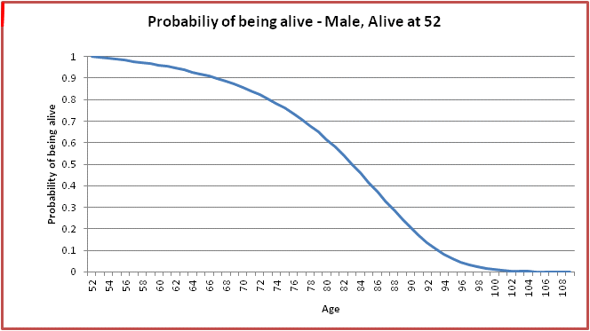
This graph can be generated by observing that the probability of being alive at n, given that the person is alive at 52 is simply:

2. The probability of death between n and n+1, given that you are an Australian male and alive at a given age. The diagram below shows this for age 52.

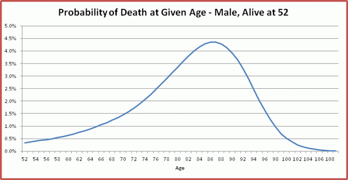
This graph can be generated by the following formula for the probability of dying between n and n+1, given the person is alive at 52:

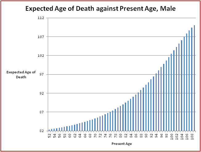
3. The expected age of death for an Australian male, given that you are alive at a certain age. For a 52 year old male, this is approx 82.4. The formula used to determine the expected age of death give you are alive at n is:

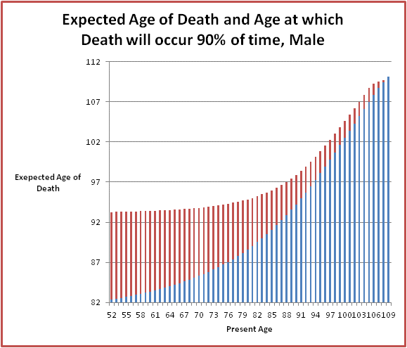
Below is the graph showing the expected age of death for an Australian male for each age from 52 onwards:

4.  The age at which an Australian male will be dead p% of the time, given that they are alive at age n. This is similar to the expected age of death. To work out this age, we need to look at the graph in point 1 above. Say for example, I am an Australian Male alive at 52, and I want to know the age at which 90% of the time I will be dead. To find this figure, we look at this graph:

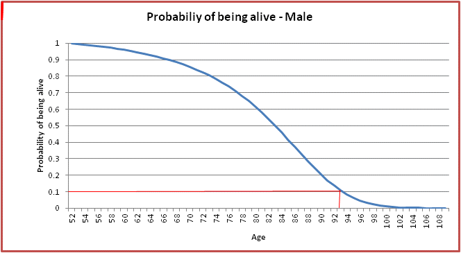
You can see from the above graph that at age 52, 90% of the time the Australian male will be dead by the age of approximately 93.

Mathematically, we choose the age n that satisfies the below:

The graph below provides this information for an Australian Male starting from the age of 52. The information is superimposed on the average age of death for reference:

OK, now have done some preliminaries, we can progress to working out spending patterns and remaining assets for the single person.

Single Person Spending Patterns and Remaining Assets

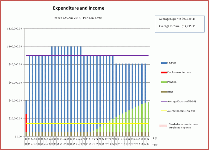
Let’s take a look at how the single person fares with the existing standard model in which we solve for running out of money at 90. Here is the latest couple spending pattern, as documented in the Mathematical Tweaks and Diversions Post:

The spending pattern for the single person is similar, except we are now using the Single Pension:

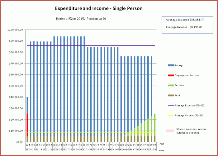
Notice that the Age Pension amount has gone down significantly, and consequently the average expense. One of the assumptions we question in this post is the validity of choosing 90 as the age at which we decide we don’t need any more money. Why was this chosen, and is it a sensible decision?

The graph below is the same graph as the graph in point 4 of the previous section, except now we have added the green line corresponding to the age of 90.

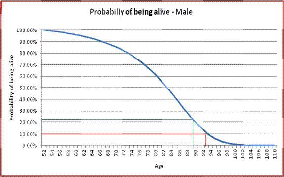
From this line we can see that there is approximately 23% chance that the retiree will be alive at 90. So, using the spending level in the above single person spending graph, there is a 23% chance that the retiree will run out of funds and be on the Age Pension only.

Rather than choosing an age at which we target to funds to run out, and then work out the probability that we will run out of funds, we can do it the other way around. That is we can chose a probability of running out of funds that we are comfortable with, and then work out the age we should target. So, for example, if I found a 10% chance of running out of funds to be more acceptable, I should target an age of just over 93 (the red line in the graph above, and also shown as the yellow line below). Settling on an age of 93, of course, would reduce the spending amount available each year as the funds would need to spread over more years.

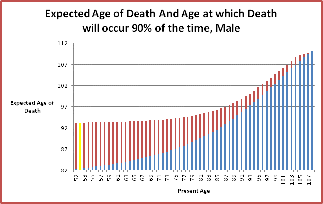
So, let’s assume I have settled on acceptable probability of running out of funds (rather than age of running out of funds), and for the sake of argument it is 10%. This tells me I should plan to live to just over 93, and I should moderate my spending to allow for this. During my second year of retirement (the first year always involves spending $40K), I spend the amount worked out by the model to spend between 53 and 54. This is shown in the diagram below (note there is some spending in year 93 as I should plan to live to approx 93.4 rather than 93):

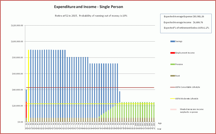
The column in yellow now becomes the spending amount for my second year of the spending plan I am generating (an adaptive spending plan).

Now let’s look at the third year of retirement. At the start of this year I still want to spend at a level that means there is only a 10% chance of running out of funds. However,  there is now a new age at which I should target to achieve this goal and it is slightly more than the original target age.This is shown as the yellow bar in the diagram below.

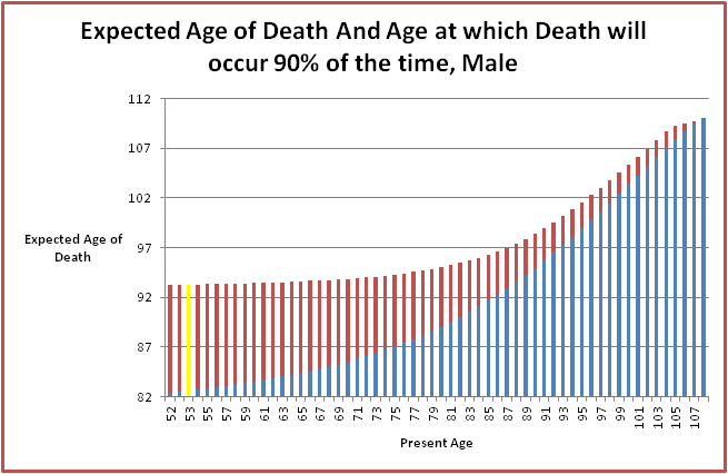
I now need to work out my spending levels again to work out what I should spend between 54 and 55, and it will be slightly less as the age that my funds (less the amount spent between 53 and 54) need to last is slightly more. This process continues over each year or retirement, with the amount to spend declining each year (slowly at first, more quickly later).

After going through the above process, the plan using 10% as the figure for the chance of running out of funds generates the adaptive spending plan shown below:

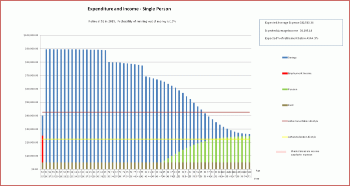
This type of plan is more sensible than the original fixed spending model, because it takes into account the fact that for each passing year that we live our expected lifespan increases. It is sensible to spread our remaining assets over a time period that takes into account our expected remaining lifespan, rather than spreading them over a period up to a fixed age (e.g. 90).

Note that I have implicitly assumed that an individual would like to maintain the same probability of running out of funds throughout their lifetime. That is, at the commencement of each year, an individual will work out the age at which they are likely to be alive with no more than, say, 10%, and divide up funds between now and then. I think this is a reasonable assumption. If an individual would like to spend a percentage amount less (e.g. 10% less at 70 and another 10% less at 80, as per above), this can be accommodated by the model as described in other sections.

Here is an animation showing how the spending pattern varies by the chosen probability of running out of funds:

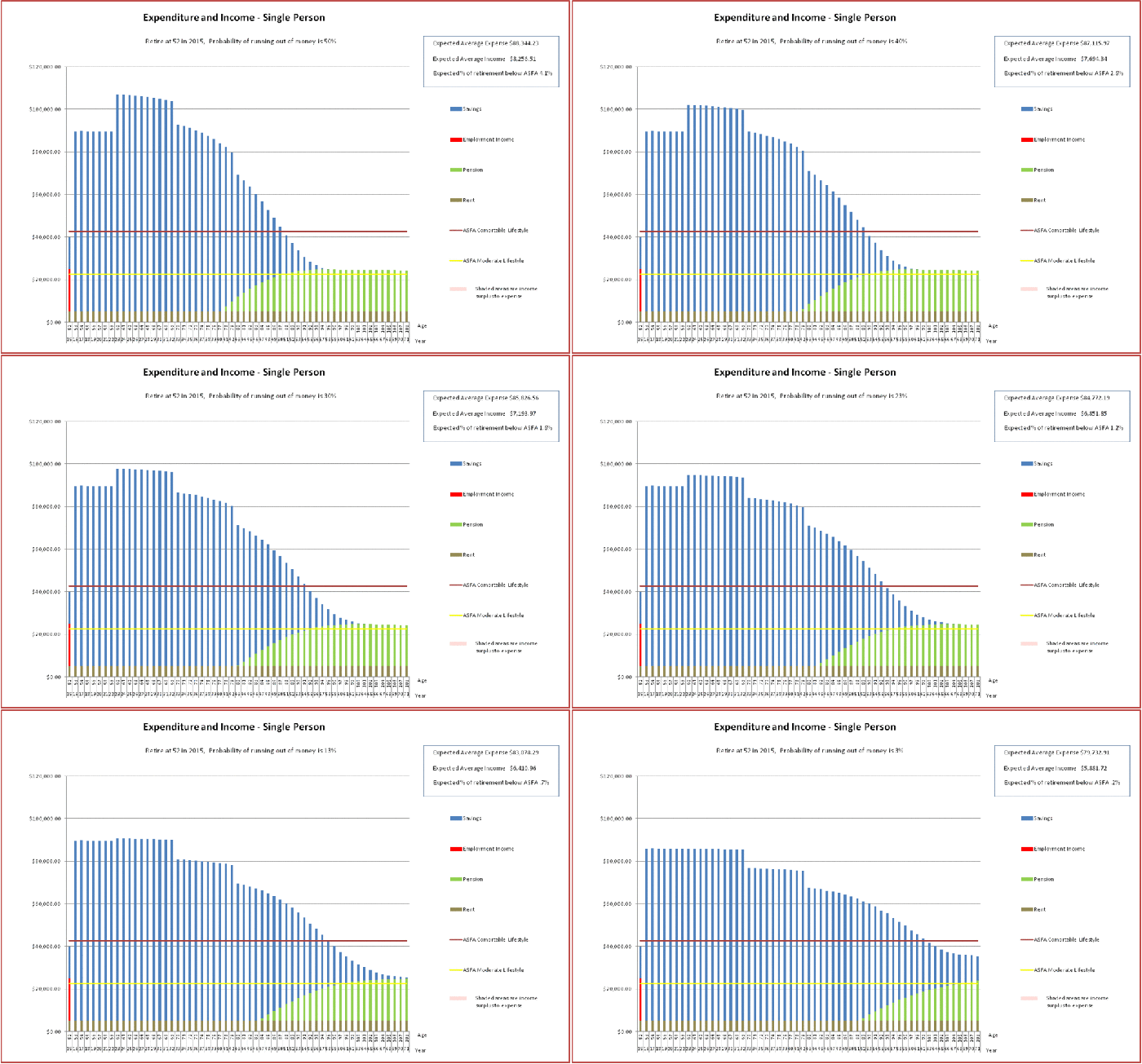
Note the “Expected Average Expense” in the top right of the above graphs. In the original fixed spending model, we worked out the spend averaged over all the years starting from the year of retirement and ending in the year we run out of funds. Now that we have mortality statistics, we can work out a more meaningful statistic, the expected average spend level, i.e. average spend levels weighted by probability of death at a given age. If E_i is the spend per year, this Expected Average expense is generated by the formula below:

In the adaptive spending plans, spending declines as we age. It no longer makes sense to think of the age at which funds run out, as we did for the fixed spend model, it now is more sensible to look at when spend levels decline below an acceptable threshold.  ASFA publish figures on the annual funds that represent a comfortable spending level for singles and couples with and without home ownership. According to this press release,  for a single person who owns their home the comfortable threshold is in early 2015, about $42.6K. Using this figure as an acceptable threshold and a probability of not running out of funds of 10%, you can see in the above diagrams that spending will not be less than the threshold until about age 96. You can also see in the mortality graph earlier in the post, that the probability of being alive at 96 is quite low (a few percent). We can also work out the expected proportion of our retirement below the ASFA threshold (or any other threshold for that matter). The diagram below shows the expected percentage of retirement below the ASFA limit and below $50K and $60K per year against the percentage probability of running out of funds. It also shows the age of falling below the ASFA limit, and the probability of falling below the ASFA limit.

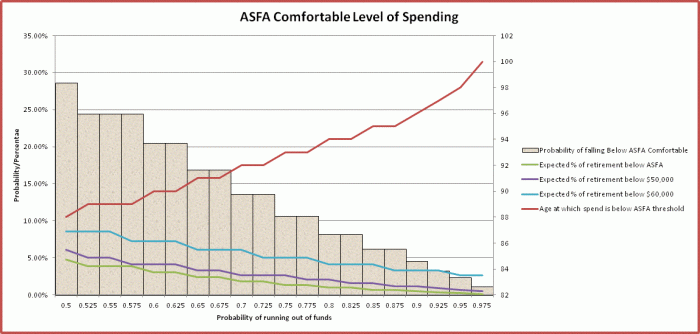
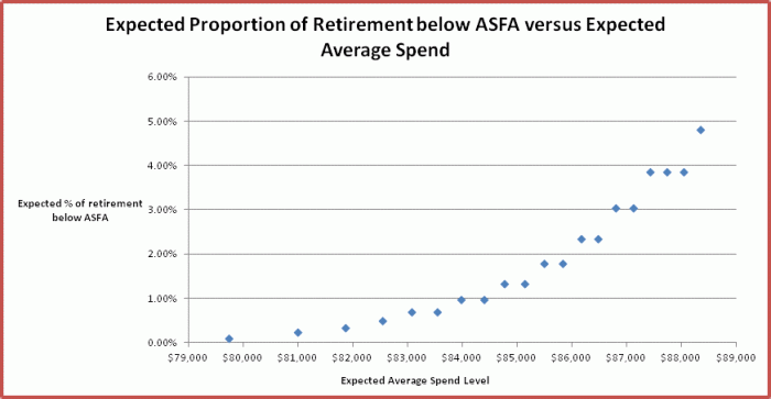
Using this diagram, if I have a certain expected maximum expected proportion of time spent below ASFA in mind, I can choose a probability on the left hand axis and see how that maps to the probability on the horizontal axis using the green line. This probability can then be used to generate a spending pattern. So, if I would like to have an expected proportion of my retirement below ASFA of no more than 0.5%, I would choose a probability of not running out of funds of 90%, and this would generate the 10% adaptive spending plan shown at the start.

Of course, the expected proportion of time spent below ASFA will increase as we age (and eventually be 100% if we live long enough).

The diagram below makes the mapping between expected proportion of retirement below ASFA with expected average spending levels more explicit:

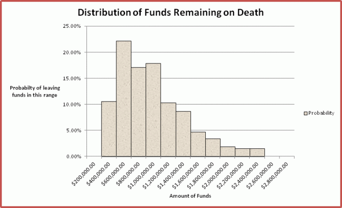
The other thing we can do now that we have mortality statistics is work out the expected value of assets left behind to beneficiaries. Because we know the amount of assets at each age for a particular spending pattern, and now know the probability of dying at that age, we can work out the amount we can expect to leave behind. The more conservative the spending pattern (the lower the probability of running out of money chosen), the more we can expect to leave behind.

For the spending pattern with a probability of running out of funds of 10%, the graph below shows the probability distribution for the amount of funds left behind:

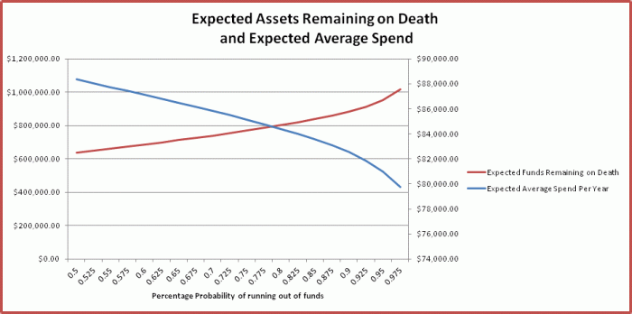
The graph below shows trade-offs between raising/lowering the probability of running out of funds chosen for your spending pattern, the expected spend level and the expected amount for beneficiaries. You can see that as the probabilities become more conservative, the expected average spending levels decline, and the expected funds remaining on death increase.

Conclusions – Mortality and the Single Person

In conclusion, in this section we have:

• Shown how we can develop a logical way of spending your funds which takes into account both your present funds, and the expected remaining duration of your life.
• Shown how this spending pattern varies in accordance with how much you value spending in the here and now versus how much you would like to avoid the possibility of living with a reduced income in later years (specifically having a high proportion of time in retirement spent below the ASFA comfortable standard). This variance is controlled by a single parameter.
• Shown that it is possible to generate a probability distribution and an expected value of funds remaining on death using the developed spending pattern and how the these vary with the above mentioned parameter.

Mortality and the Couple

OK, now that we have looked at using mortality statistics to gain financial insights into the spending levels during retirement for a single person, let’s now look at the married couple.

To begin with, we will look at some mortality graphs which will be of assistance when working out spending patterns and assets.

Couple Mortality Statistics

We can work out the following related to couple mortality:

1. Most people know that females, on average have a longer life expectancy than males. Not only that, but in most partnerships, the female is usually a few years younger than the male. Put these together and the female partner will usually end up outliving the male by quite a bit. The below graph shows the probability of being alive for subsequent years for a 52 year old Australian male and a 52 year old Australian female.

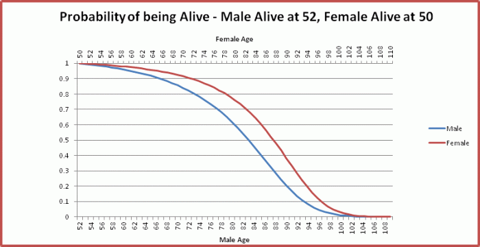
2. The below graph shows the probability of each person in the partnership being alive assuming that the male is two years older, the male is 52, and the female is 50:

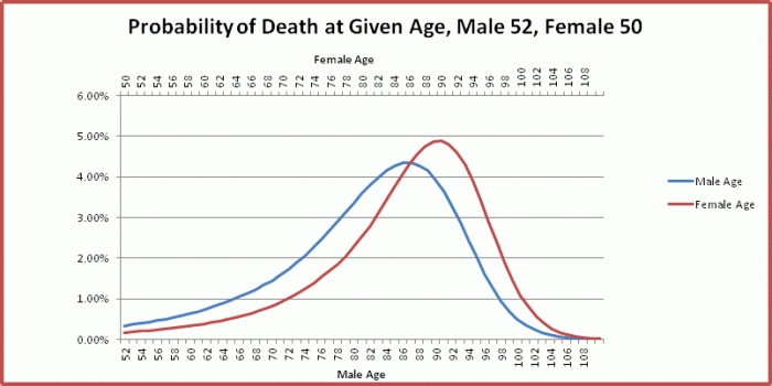
3. The below graph shows the probability of death between n and n+1 for both the male and female, assuming the male is 52 and two years older than the female. You can see that the death rates for the female occur quite a bit later than the male.

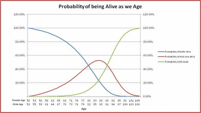
4. The below graph provides some information on likelihood of both partners being alive, one only alive and both dead, assuming the male is 52 and the female is 50. Interestingly by the time the male is about 81 there is a 50% chance that one one of the couple has died. Note that the age pension  shifts down to the single pension when one of the couple dies, so the couple spending patterns that have used the assumption of the couple pension until 90 are not really realistic.

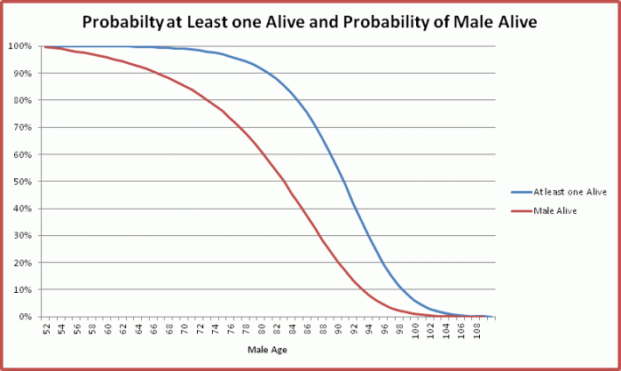
5. Here is a graph which compares the probability of at least one partner in the couple being alive against the probability of the male being alive. You can see there is quite a difference. Because spending occurs while  the couple or a single person survives, we can expect quite a bit of reduction in the expected beneficiary amount when comparing the couple with the single person.

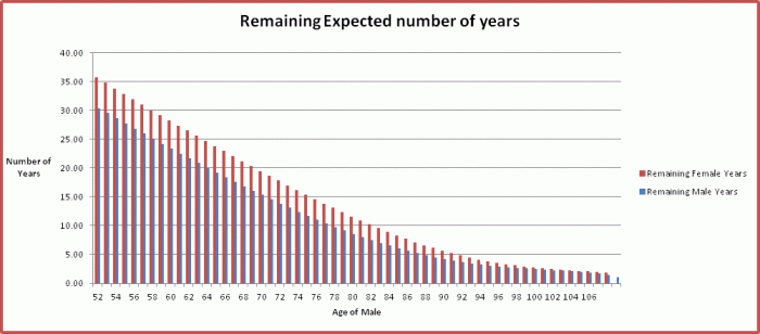
6. Lastly here is a graph showing the expected number of years to live for a couple proceeding through retirement with the male age 52 and female age 50. You can see that the female has quite a few more years than the male.

Couple Spending Patterns and Remaining Assets

Now let’s look at how we can use mortality statistics to work out appropriate spending levels for the couple, and also determine the expected assets remaining. We will use the same kind of ideas as used for the single person. However, for the couple, it is a bit more complex as we need to take into account all the possible combinations of the age of death of each person in the couple.

Firstly, each member of the couple will need to choose a probability of running out of funds which is acceptable to themselves. This will be used when the other member of the couple dies, i.e. when they become single. This is a personal choice and reflects how much the individual values spending in the here and now versus reducing spending now in favour of conserving savings that could possibly be used in the future. Information on how this can be chosen is discussed in the first part of this post.

Secondly we need to work out the spending levels while a couple. To work out these values, two factors need be agreed on by the couple, by mutual consensus. These are:

1. The planned spending level, in terms of a percentage of the spending level for the couple, for the surviving partner. Costs for a single person will be less than for a couple, but more than 50%. 60% might be a reasonable figure and and I have used this figure as the default figure in this post.
2. An agreed acceptable percentage probability of running out of funds, assuming a constant spend while a couple, and a constant spend for the surviving partner in accordance with the percentage above. Note that “running out of funds” means that, using the planned spending levels above, at least one member of the couple is alive at the time that all funds run out. I will use 20% for my default here.

These two numbers are used to determine the spending levels of the couple while they are a couple. Some strategies used to select these numbers are to choose numbers that sound reasonable, to use the default values as mentioned above, or to look at graphs showing how various parameters (such as expected proportion of retirement below ASFA levels) vary as we change them. This latter option is explored later in the post.

Now we will look into how we can generate couple spending levels. Note that by using the couple spending rules above, we can work out, for a particular level of spending, which age combinations of death  will have funds remaining, and which will result in running out of funds. In general, the longer we live or the higher our spending level, the more likely we are to run out of funds. As we know the probabilities of each of the age combinations of death, we can work out the probability of running out of funds for a particular spending level. We want the maximum spending level possible, while still ensuring that the probability of running out of funds for either member of the couple is less than the couple nominated amount. This determines the spending level to be used as the beginning of a year.

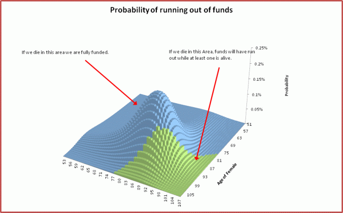
The diagram above provides some more information on this approach. It shows the probabilities of all the possible combinations of ages of death for the couple (starting from the male age of 52), and is colour coded to show in which of these we run out of funds given a proposed spending level. The area colour coded in green is the area in which we do run out. The sum of probabilities in this area is less than 20%. The spending level is chosen as the maximum level possible while still keeping the green area less than 20%.

In keeping with the techniques used for the single person, we want the amount to be spent to be adaptive. That is, it varies each year into retirement based on the additional information that we are both alive. The spending level for a couple in our situation, with the choice of 20% for the probability of not running out of funds for either of us, and a value of 60% to be used for as the percentage of spend for the surviving partner is shown below.

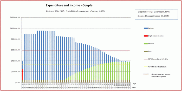
Note the similarity with the adaptive spending plan for the single person. Each point on this graph has the property that, moving forwards, if we spend at the nominated level while a couple, and at 60% of this value when one member of the couple dies, then we can expect that there is no more than a 20% chance that either person in the couple will run out of money (i.e. both will die before the funds are depleted). In addition, the spend level is the maximum level that has this property.

Now that we have the spending levels while we are a couple, the next thing to do is to work out the spending levels when one of us becomes single. Now we just use the same approach as the first section in this post, i.e. the approach used for the single person, using the percentage of not running out of funds nominated by that person.

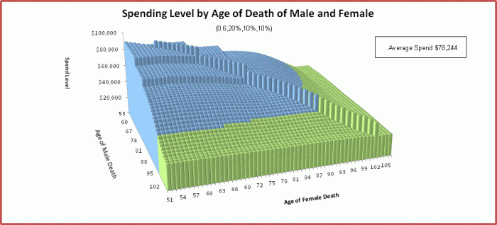
Here is the graph which shows the spending level at each age combination, including the couple spend levels already worked out:

The graph below should help with understanding this diagram:

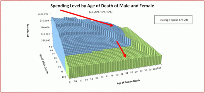
When you are a couple you proceed down the first red line in the above diagram. That is you spend at the rates down the diagonal spike in the middle of the graph. When one partner in the couple dies (shown in the above as the female partner dying at approx 86), the remaining person in the couple spends in accordance with the second red line.

Note that:

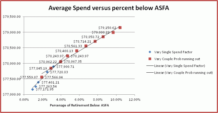
• The total average expected spend can be worked out in a similar way to that used with the single person i.e. by working out the average spend for each combination of death, multiplying by the probability of this combination and summing. In this case, it is approx $79K, which is quite low.
• The diagram is colour coded showing  which age combinations are above (blue) or below (green) the ASFA comfortable spending levels (taking into account if we are a single or a couple at the time).
• By summing up all the probabilities that are blue, you can work out the likelihood of not falling below the ASFA comfortable spending level. In this case it is 59%, which is not that high! You can also work out the proportion of retirement expected to be below ASFA for both members of the couple, the male and the female (again using a similar technique used to calculate the average spend). In this case it is 4.27%, 3.1%.  and 4.77% respectively. As you might have expected, the female, due to her longevity, is expected to have the highest proportion below ASFA.
• You can see that on most occasions the spend rate for the couple is higher than the single. The reason for this is:
  • We are planning for the single person to have a spend of 60% of the couple.
  • The differences in the conservativeness of the single spending plan and the couple spending plan. If for example, the single spending plan is quite conservative, we would expect a lower spend than the spend that is used by the couple at the same age.
• Note that if the female dies early then the male spend level is just as high as the couple. The reason for this is that the male has more funds than necessary to get through the average lifespan, because the spend level for the couple takes into account the longer lifespan of the female. This counters the lower single age pension.
• While the diagram looks symmetric, it is not because the female and male partners have different mortality statistics, and therefore different spending patterns. Also if there was a large gap in age between members of the couple, the diagram would be much more asymmetric.

Here is the spend diagram from another perspective, this time showing the lower spend of the female:

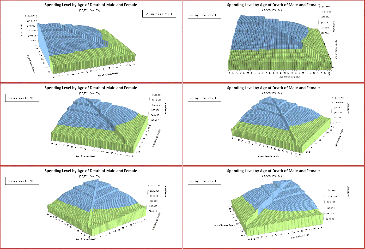
We can also work out average spending levels in a few different ways

Average spending while we are a couple: $86,949

Average spending for Female when Single: $49,677

Average spending for Male when Single: $56,486

Overall average spending for Female: $76,062

Overall average spending for Male: $81,162

Overall average spending: $78,244

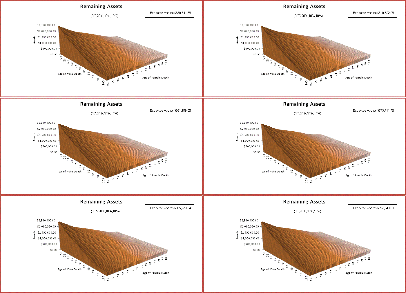
Here is a diagram showing the assets for each combination of age of death:

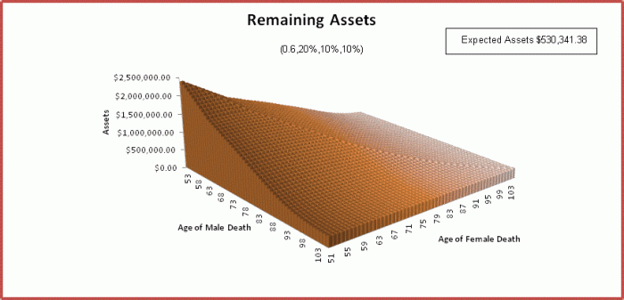
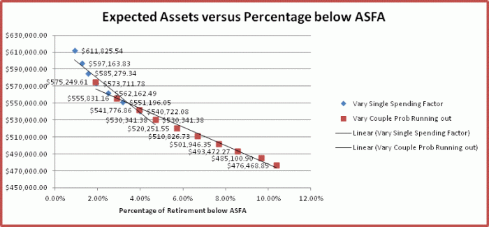
We can weight this by the probability of each combination of age of death to determine the expected value of assets remaining on death.  In this case it is approx $530K.

Working out the best parameters for the couple

In this section we see how the spending patterns are affected by changing the chosen probability of running out of funds as a couple, and the chosen percentage of couple spend chosen for the single. This is done by showing how the spending patterns visibly change as we modify the parameters.

Varying the Single Spending Percentage

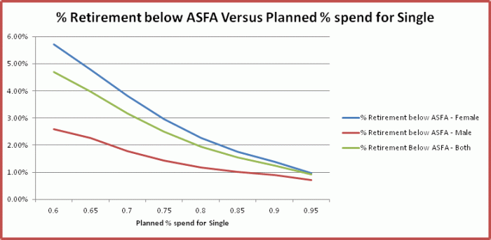
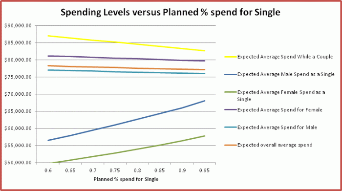
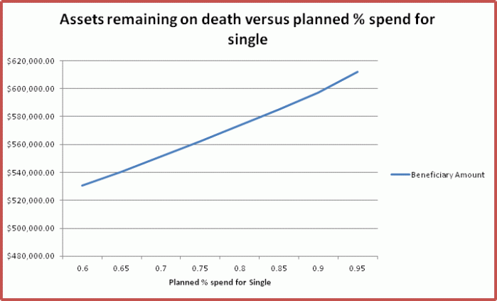
The factor we use for the single spending when working out the couple spending model is a bit mysterious. When this factor is low (e.g. 60%) it tends to:

• Increase our spending while a couple and decrease it while we are a single.
• Increase the expected proportion of retirement spend under ASFA
• Increase in the overall spend
• Reduce the expected value of assets left to beneficiaries.

If you especially value your time while a couple (which I do!), I recommend a low value for this figure.

The graph below shows how the overall spending changes with this parameter is shown below.

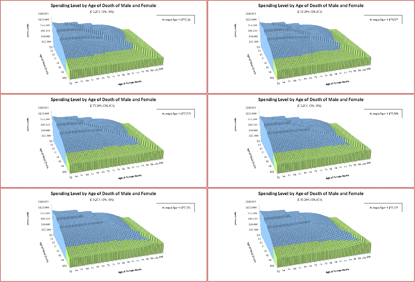
This graph shows how the assets change with this parameter (not a great deal!):

These graphs provide more aggregate information for the changes. This one shows how the % of time spend below ASFA varies with the figure.

This one shows the how the spend levels vary:

This one shows how the expected assets remaining for beneficiaries vary:

Varying the probability of running out of funds for the couple

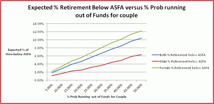
OK, now we can look at varying the percentage probability of running out of funds for the couple. We expect that by increasing this we would see an

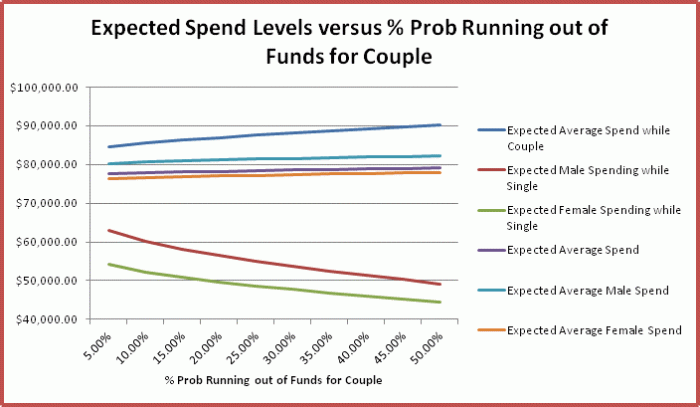
• Increase in the couple spend,
• Increase in the overall spend,
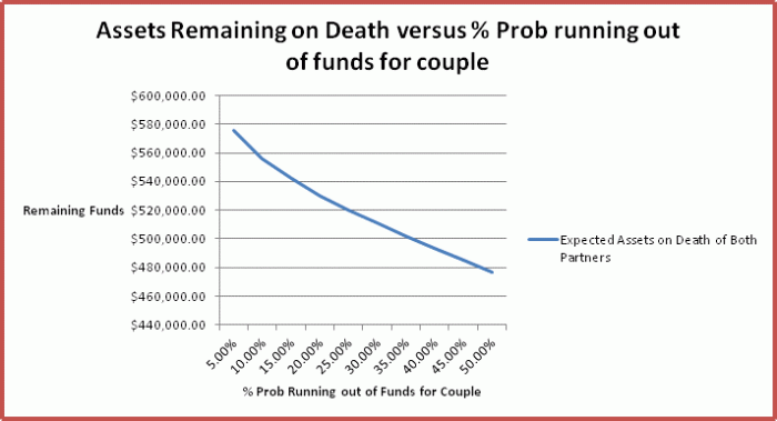
• Reduction in the amount of funds left to beneficiaries
• Increase in the expected amount of time spent under ASFA

In other words, much like a reduction in the Single spending percentage. This figure should be increased if you prefer to spend in the here and now, and are less concerned with preserving funds for the later years of retirement.

Let’s see if our predictions bear out. I have kept the percentage spend of the couple spend for the single person fixed at 60%, and the single probability of running out of funds fixed at 10%,

Here is the graph showing how the % of time spend below ASFA varies with the couple prob of running out of funds. As expected, this proportion increase as the couple probability increases.

And here is the graph showing how spending levels vary. As expected, spend levels for the couple and overall spending increase, although the latter not significantly so. Single spending levels decline quite a bit.

And here is the graph showing how expected assets remaining for beneficiaries vary. As expected they decline as the % prob of running out of funds for the couple increases.

Combined Scatter Diagrams

Finally here are the combined scatter diagrams:

Why have our spending levels and Assets to beneficiaries dropped

You can see from the original overall spending graph and the previous section, average spending levels have dropped by about $10K (or about 11%) when compared with the original couple spending model, and also the amount of funds left by the couple to beneficiaries has dropped about $350K (or about 42%) when compared to the amount left by the single person. Why is this?

The average spend has reduced because:

• In the new model, the couple must set aside funding for future years every year while in the original model we only set aside funds until 90.
• In the new model, it is expected that in many years the Single Pension will be used rather than the higher couple pension. In the original model, the couple pension was used at all times.

The average spend is increased because:

• We are now averaging the expected spend as weighted by age of death. The lower spend in later years will be given less weighting.

The expected funds left to beneficiaries is reduced because:

• We now have a couple spending money and reducing the remaining funds available on death. When one partner dies, the other partner continues to spend. The average lifespan of the combined partner entity is significantly longer than the male individual.

Conclusions

Working out spending levels while incorporating mortality statistics has been a lot of work! Probably more than the rest of the blog combined. Is going to this level of complexity and detail worth it?

I think it is, for these reasons:

• Previously we just chose an age at which we wanted our funds to last. This choice didn’t relate to anything meaningful, such as the expected percentage of retirement spent below the ASFA retirement standard. With mortality statistics we can select a spending pattern which relates to something real.
• Previously we spent the same amount right up to the age at which we chose to run out of funds. This is not realistic behaviour because any rational person would reduce their spend when they realize that there is a good chance of exceeding this age. You can use mortality statistics to work out how you should reduce your spend to anticipate this possibility.
• Previously we had no idea how our spending plan would impact on the amount of funds we are likely to leave beneficiaries. With mortality statistics, we see how the expected value of funds left to beneficiaries relates to the the spending pattern adopted.
• When we use mortality statistics the estimated average spend is different than the spend worked out previously. In fact under most circumstances it will be lower. This additional information may help to determine a good time for retiring.