More on Risk

Monte Carlo Simulations

In a previous post I said I wouldn’t do any more graphs, but I couldn’t resist. In this post I look at using simulated Super returns to generate distributions of key retirement variables. I look at two situations:

1. The impact of variable Super returns on the distribution of the age at which the funds run out, assuming a constant spend.
2. The impact of variable Super returns on the distribution of average spend, assuming that spending is moderated each year in accordance with the level of assets (as described in the “Retirement Calculations”).

Normal Distributions and Returns

In this post I will assume that Super returns are normally distributed, and the return from one year is independent of returns from other years. It is common to make this type of assumption when trying to model stochastic variables, and I believe a reasonable assumption in this case. I have found some evidence that this assumption has been made by funds when trying to develop risk models, for example here:

http://www.rest.com.au/getdoc/71b3d709-afab-4890-83d2-f4f5fba15e79/Standard-Risk-Measure-Methodology

This site discusses some aspects relating to this assumption:

“Normal Distribution – Asset class returns are assumed to be normally distributed (i.e. they have a standard bell shaped distribution with a peak at the mean).  This assumption is a simplification of reality and assumes zero skewness.  This means that returns are symmetrically distributed around the mean. (Negative skewness means there is a substantial probability of a big negative return; positive skewness means that there is a greater-than-normal probability of a big positive return.)  The other limitation of a normal distribution is that it has no upper and lower bounds (i.e. it is possible to have a negative return greater than 100% which would not normally be the case without the use of leverage).”

Further study would be required to assess the validity of this assumption.

As for the standard deviation that is applicable to Australian Super fund returns, the document below looks at returns and volatility of Australian Superannuation funds between 1995 and 2002:

Click to access the-investment-performance-of-australian-superannuation-funds-feb-2003.pdf

One of the conclusions is:

“For the sample of funds submitting annual returns in the seven years to 2002, the average fund has an annual net return on assets (ROA) of 6.69%, volatility of 6.21% and annual expense ratio (ER) of 1.28%.”

Note that the Volatility is the standard deviation of returns.

I will assume a real pre-tax Superannuation return of 3.25% (i.e. pre-inflation), or about 5.5% prior to 60 and 6.0% after 60 (after inflation), in accordance with my original model, and that the volatility is 6.21% in accordance with the above mentioned paper. Note that the Standard deviation of the Australian Super Balanced option for returns over the last 17 years is about 7.5%

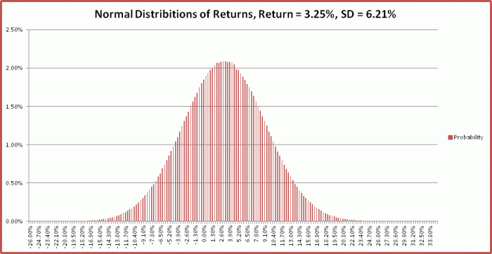
I used Excel to generate a normal distribution under these assumptions (using 64000 simulations, each containing about 50 years of random normal returns) using a random number generator and the NORMINV function. The below graph shows the result:

Impact of variable Super returns on when funds run out, assuming a constant spend

Now if I use the data points in the Normal distribution generated in the previous section and run through 64000 simulations using the spend I recommended in my post “Tweaks and Mathematical Diversions” (about $89K), I get the distribution of age of funds running out shown in the diagram below.

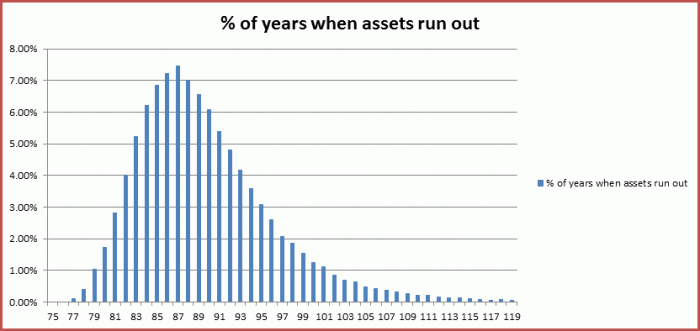
The average age is about 90.36, and the standard deviation is about 5.7.

If I look at cumulative probabilities, I get the diagram below:

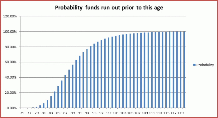
These two graphs are saying that there is around a 50% chance that we will run out of funds prior to 90, and a 20% chance that we will run out of funds prior to 85, assuming a constant spend at the level that is recommended if we want assets to run out at 90.

Impact of variable Super returns on spend, assuming that spending is moderated each year

In this section I look at the distribution of average spend, assuming that each year we modify our spending habits in light of the amount of funds remaining at the end of the previous year. This uses the approach described in the “Retirement Calculations” post whereby the amount to be spent in a given year is the amount which causes the assets at age 90 to be zero, assuming standard returns and inflation.

Unfortunately in this case it is difficult to run through so many trial runs as each run is computational intensive (as it involves 38 optimizations). For the moment I have done 9000 runs. I have also used my pre-tweaked model so that I could compare the results with earlier posts in the blog ( a spend of $87K).

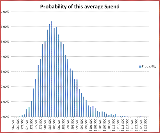
Here is the result:

Not that this is not as smooth as the other graphs due to the limited number of runs. Also, although the average is $87,600, this is skewed by some high values, and the median is about $1000 lower. The standard deviation is about $7000.

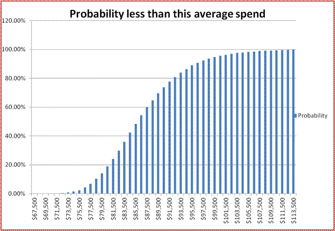
Here is the graph showing the probability of less than a given spend:

Conclusions

In conclusion:

• It is possible to use Monte Carlo simulation techniques to generate distributions of the numbers of years savings will last into retirement, under the assumption that Super returns are normally distributed, and Super returns each year are independent of all other years. The resulting graph can provide an indication of the riskiness of the proposed spending levels, and the probability that Super funds may run out prior to any given age.
• It is also possible to use Monte Carlo simulation techniques to generate distributions of average spend given that spend is moderated each year according to the performance of Super, again assuming Super funds are normally distributed and each year’s performance is independent of others. The resulting graph can be used provide an indication of the riskiness of commencing retirement given a certain asset base, and can provide the probability that your average spending levels will be below a given amount.